Chapter 7: Alternating Current

Dear Class 12 Student! The electric power that runs our homes, powers factories, charges our devices, and energizes entire cities is Alternating Current (AC). Building upon Electromagnetic Induction (Chapter 6), this chapter bridges physics and higher-level trigonometry. From understanding why household supply is labeled $220\text{ V}$ to mastering Series LCR Resonance, Phasor Diagrams, Power Factors, and Transformers, these notes provide a complete, step-by-step foundation with full mathematical derivations and physical reasonings for CBSE Boards & JEE/NEET!

1. Introduction to Alternating Current (AC vs DC)

Electric current can flow in two fundamental forms depending on how its magnitude and direction behave over time:

Direct Current (DC): Current that flows in a single constant direction with a constant or varying magnitude. Sources include electrochemical cells, batteries, and DC generators.
Alternating Current (AC): Current whose magnitude changes continuously with time and whose direction reverses periodically. Sources include AC generators (dynamos) and power plant alternators.

Parameter	Direct Current (DC)	Alternating Current (AC)
Direction	Unidirectional (Single direction)	Reverses direction periodically
Frequency ($f$)	$0 \text{ Hz}$ (Constant)	$50 \text{ Hz}$ (India) / $60 \text{ Hz}$ (USA)
Long Distance Transmission	High power loss as heat ($I^2R$)	Transmitted at very high voltage with minimal power loss
Voltage Stepping	Cannot be stepped up/down easily	Easily stepped up or down using Transformers

Physical Reasoning: Why AC is Preferred for Power Grids Power generated at power stations must travel hundreds of kilometers to reach cities. Electric power loss in transmission lines is given by Joule Heating: $P_{\text{loss}} = I^2 R$.
By using a Step-Up Transformer at the power generator, the voltage $V$ is increased by a factor of 100. Since Power $P = V I$ is constant, increasing $V$ reduces current $I$ to $\frac{1}{100}\text{th}$ of its original value. Consequently, power loss $I^2R$ is reduced to $\frac{1}{10,000}\text{th}$ (or $0.01\%$)! At local sub-stations, a Step-Down Transformer safely reduces the voltage back down to $220\text{ V}$ for home use. This is impossible with DC!

Mathematical Expression for Sinusoidal AC

An alternating voltage produced by rotating a coil of $N$ turns and area $A$ in a uniform magnetic field $B$ at angular speed $\omega$ is represented by a sine function:

Sinusoidal Equations Instantaneous Voltage: $$v = V_m \sin(\omega t + \phi_0)$$ Instantaneous Current: $$i = I_m \sin(\omega t + \phi_0)$$

Instantaneous Value ($v, i$): The magnitude of voltage or current at any specific instant of time $t$.
Peak Value / Amplitude ($V_m, I_m$ or $V_0, I_0$): The maximum numerical value reached by AC in either positive or negative half-cycle.
Time Period ($T$): The time taken to complete one full cycle of oscillation ($T = \frac{2\pi}{\omega}$).
Frequency ($f$ or $\nu$): The number of complete cycles executed per second ($f = \frac{1}{T} = \frac{\omega}{2\pi}$). Standard mains frequency in India is $50\text{ Hz}$ (reverses direction 100 times per second!).
Angular Frequency ($\omega$): The rate of change of phase angle ($\omega = 2\pi f = \frac{2\pi}{T}$, Unit: $\text{rad/s}$).
Phase Angle ($\omega t + \phi_0$): Represents the fractional state of completion of a wave cycle at time $t$.

2. Average (Mean) and RMS Values of AC

Conceptual Question: Why do Standard DC Meters Fail for AC? Standard moving-coil ammeters and voltmeters work on the principle of magnetic torque $\tau = N I A B$. Since AC reverses direction every half cycle, the average magnetic torque over a complete cycle is exactly zero ($\tau_{\text{avg}} = 0$). As a result, the pointer of a DC meter fluctuates so fast that due to inertia it remains stuck at zero!
Solution: AC ammeters and voltmeters are designed based on the heating effect of current ($H \propto I^2$). Since $I^2$ is always positive regardless of current direction, these hot-wire instruments deflect proportional to $I_{\text{rms}}^2$ and directly measure RMS values!

A. Mean (Average) Value of AC ($I_{\text{avg}}$ or $I_{\text{mean}}$)

1. Over a Complete Cycle:
The average value of AC over one full cycle ($0$ to $T$) is defined as:

$$\begin{aligned} I_{\text{avg, full}} &= \frac{1}{T} \int_0^T I_m \sin\omega t \, dt = \frac{I_m}{T} \left[ \frac{-\cos\omega t}{\omega} \right]_0^T \\ &= -\frac{I_m}{\omega T} [\cos(2\pi) - \cos(0)] = -\frac{I_m}{2\pi} [1 - 1] = \mathbf{0} \end{aligned}$$

Thus, the average value of AC over a complete cycle is always zero because the area of the positive half-cycle perfectly cancels the area of the negative half-cycle.

Full Derivation: Mean Value of AC Over a Half Cycle Definition: The mean value of AC over a half cycle ($0$ to $T/2$) is defined as that steady direct current ($I_{\text{avg}}$) which transfers the same amount of charge through a circuit in time $T/2$ as is transferred by the alternating current in the same time.

Charge transferred by AC in small time $dt$: $dq = i \, dt = I_m \sin\omega t \, dt$.
Total charge transferred in positive half cycle ($0$ to $T/2$): $$\begin{aligned} Q &= \int_0^{T/2} I_m \sin\omega t \, dt = I_m \left[ \frac{-\cos\omega t}{\omega} \right]_0^{T/2} \\ &= -\frac{I_m}{\omega} \left[ \cos\left(\omega \cdot \frac{T}{2}\right) - \cos(0) \right] \end{aligned}$$ Substitute $\omega = \frac{2\pi}{T}$: $$\begin{aligned} Q &= -\frac{I_m}{2\pi / T} \left[ \cos\left(\frac{2\pi}{T} \cdot \frac{T}{2}\right) - 1 \right] = -\frac{I_m T}{2\pi} [\cos\pi - 1] \\ &= -\frac{I_m T}{2\pi} [-1 - 1] = \frac{2 I_m T}{2\pi} = \mathbf{\frac{I_m T}{\pi}} \end{aligned}$$ By definition of steady average current: $Q = I_{\text{avg}} \times \frac{T}{2}$.
Equating both expressions: $$I_{\text{avg}} \cdot \frac{T}{2} = \frac{I_m T}{\pi} \implies \mathbf{I_{\text{avg}} = \frac{2 I_m}{\pi} \approx 0.637 I_m}$$ Similarly, average voltage over a half cycle: $$V_{\text{avg}} = \frac{2 V_m}{\pi} \approx 0.637 V_m$$

B. Root Mean Square (RMS) Value of AC ($I_{\text{rms}}$ / $V_{\text{rms}}$ or $I_{\text{eff}}$ / $V_{\text{eff}}$)

Concept: Since average current over a full cycle is zero, we define the effective strength of AC based on its thermal (heating) capability.

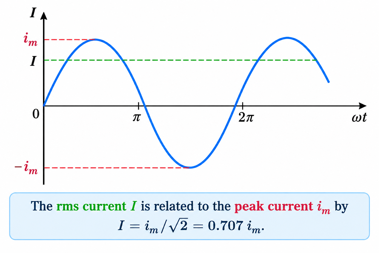
Sinusoidal Current RMS Relationship Diagram

Full Derivation: RMS Value of AC (Must-Know Board Derivation) Definition: The Root Mean Square (RMS) value of AC is defined as that steady direct current ($I_{\text{rms}}$) which produces the same amount of heat in a given resistance $R$ in a given time $T$ as is produced by the AC in the same resistance in the same time.

Heat produced by AC $i = I_m \sin\omega t$ in small time $dt$: $dH = i^2 R \, dt = (I_m \sin\omega t)^2 R \, dt$.
Total heat produced over one complete cycle ($0$ to $T$): $$\begin{aligned} H &= \int_0^T I_m^2 R \sin^2\omega t \, dt = I_m^2 R \int_0^T \left( \frac{1 - \cos 2\omega t}{2} \right) dt \\ &= \frac{I_m^2 R}{2} \left[ \int_0^T dt - \int_0^T \cos 2\omega t \, dt \right] \\ &= \frac{I_m^2 R}{2} [ T - 0 ] = \frac{I_m^2 R T}{2} \end{aligned}$$ By definition, if $I_{\text{rms}}$ is the steady current producing the same heat $H$ in time $T$: $$H = I_{\text{rms}}^2 R T$$ Equating the two heat expressions: $$I_{\text{rms}}^2 R T = \frac{I_m^2 R T}{2} \implies I_{\text{rms}}^2 = \frac{I_m^2}{2}$$ Taking square root on both sides: $$\mathbf{I_{\text{rms}} = \frac{I_m}{\sqrt{2}} \approx 0.707 I_m} \quad \text{and} \quad \mathbf{V_{\text{rms}} = \frac{V_m}{\sqrt{2}} \approx 0.707 V_m}$$

Form Factor & Peak Factor

Form Factor: Ratio of RMS value to Average value over half cycle: $$\text{Form Factor} = \frac{V_{\text{rms}}}{V_{\text{avg}}} = \frac{V_m / \sqrt{2}}{2V_m / \pi} = \frac{\pi}{2\sqrt{2}} \approx \mathbf{1.11}$$
Peak (Crest) Factor: Ratio of Peak value to RMS value: $$\text{Peak Factor} = \frac{V_m}{V_{\text{rms}}} = \frac{V_m}{V_m / \sqrt{2}} = \sqrt{2} \approx \mathbf{1.414}$$

Real-World Application: Why $220\text{V}$ AC is More Dangerous than $220\text{V}$ DC When a household electrical rating says $220\text{ V}$ AC, it ALWAYS refers to the RMS Voltage ($V_{\text{rms}}$).
The actual maximum peak voltage hitting the appliance (and a person touching the wire) is: $$V_m = V_{\text{rms}} \times \sqrt{2} = 220 \times 1.414 = \mathbf{311.08 \text{ V}}$$ Thus, a $220\text{V}$ AC line oscillates between $+311\text{V}$ and $-311\text{V}$ (a peak-to-peak swing of $622\text{V}$!), whereas a $220\text{V}$ DC line remains constant at $220\text{V}$. Hence, AC is much more dangerous than DC of the same nominal voltage!

3. Representation of AC by Rotating Vectors (Phasors)

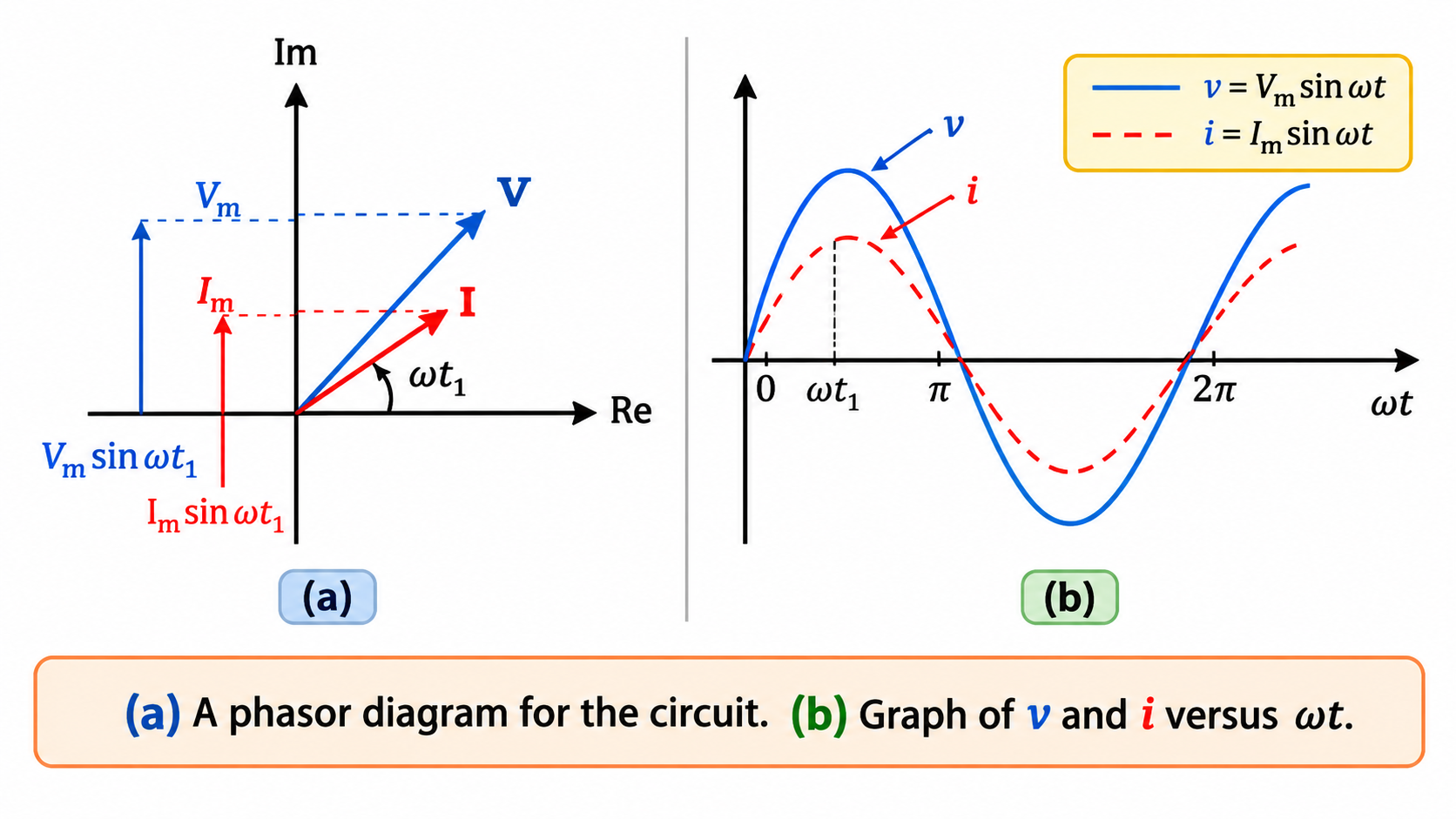
Since sinusoidal alternating voltages and currents oscillate periodically with time, analyzing complex AC circuits using standard sine/cosine equations becomes tedious. Instead, we use Phasor Diagrams.

What is a Phasor? A Phasor is a vector of magnitude equal to the peak amplitude ($V_m$ or $I_m$) of an alternating quantity, rotating counterclockwise about the origin with constant angular velocity $\omega$.

Key Properties:

The length of the phasor vector represents the peak amplitude ($V_m$ or $I_m$).
The angle made by the phasor with the positive X-axis at time $t$ represents the phase angle ($\omega t$).
The projection of the phasor on the vertical Y-axis gives the instantaneous value of voltage ($v = V_m \sin\omega t$) or current ($i = I_m \sin\omega t$).

4. AC Voltage Applied to Pure Components (R, L, C)

A. Pure Resistor (R)

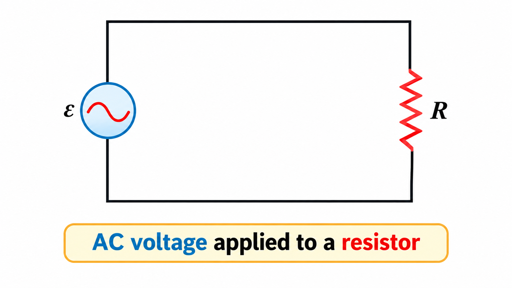
Consider an AC source $v = V_m \sin\omega t$ connected across a pure resistor of resistance $R$.

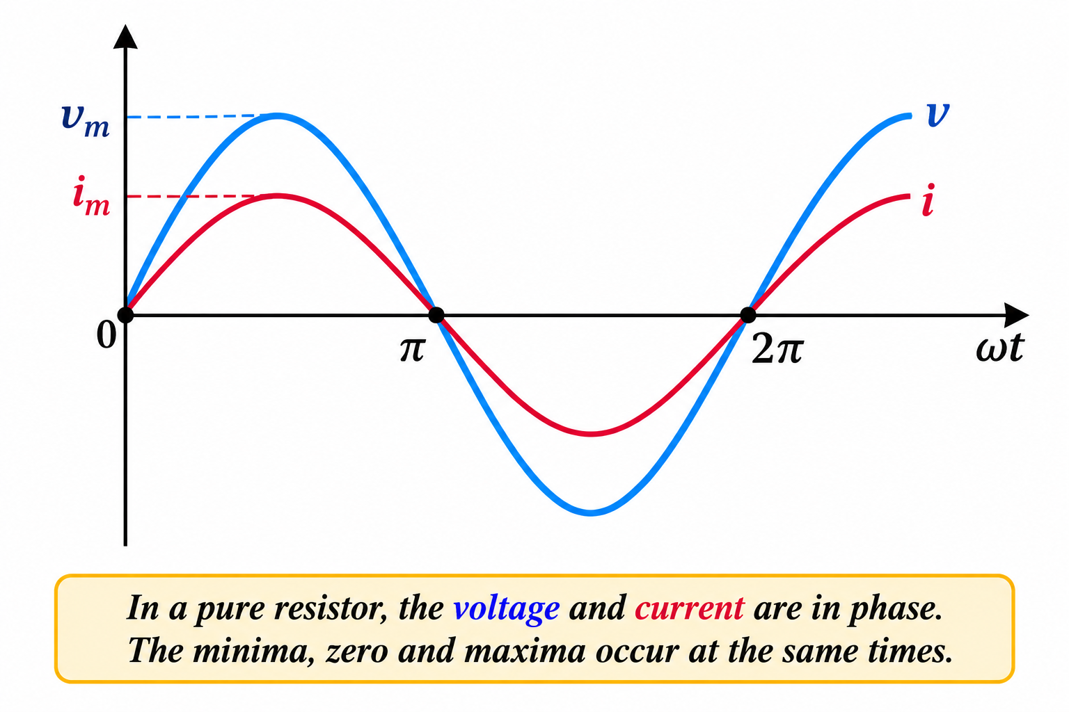
AC Voltage Applied to a Resistor Circuit Diagram

By Kirchhoff's Voltage Law (KVL): $v - i R = 0 \implies i = \frac{v}{R} = \frac{V_m}{R} \sin\omega t = \mathbf{I_m \sin\omega t}$ where $I_m = \frac{V_m}{R}$.

Phase Difference ($\phi$): $\phi = 0^\circ$. Voltage and current are in phase. Both reach maximum, zero, and minimum simultaneously.
Opposition: Resistance $R$ (Unit: $\Omega$). $R$ is independent of frequency $f$.

Phasor Diagram and AC Waveforms for Pure Resistor

B. Pure Inductor (L)

Consider an AC source $v = V_m \sin\omega t$ connected across a pure inductor of self-inductance $L$ and zero resistance.

Full Derivations: Pure Inductor & Inductive Reactance As alternating current flows through the inductor, its magnetic flux changes, inducing a self-back EMF: $e = -L \frac{di}{dt}$ (Lenz's Law).
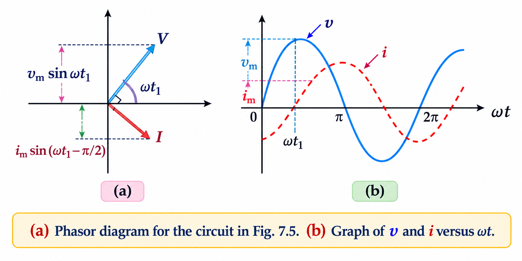
Applying KVL to the closed circuit: $$\begin{aligned} v + e = 0 &\implies V_m \sin\omega t - L \frac{di}{dt} = 0 \\ &\implies \frac{di}{dt} = \frac{V_m}{L} \sin\omega t \end{aligned}$$ Integrating both sides with respect to time $t$: $$\begin{aligned} i &= \int \frac{V_m}{L} \sin\omega t \, dt = \frac{V_m}{L} \left( \frac{-\cos\omega t}{\omega} \right) \\ &= -\frac{V_m}{\omega L} \cos\omega t = \mathbf{I_m \sin\left(\omega t - \frac{\pi}{2}\right)} \end{aligned}$$ where $I_m = \frac{V_m}{\omega L}$.
The term $\omega L$ opposes current flow and is called Inductive Reactance ($X_L$): $$\mathbf{X_L = \omega L = 2\pi f L}$$

Phase Relation: Current lags voltage by $90^\circ$ ($\pi/2\text{ rad}$). Voltage reaches peak $T/4$ seconds before current.
Physical Reason for $X_L \propto f$: Higher frequency means current changes at a faster rate ($\frac{di}{dt}$ is larger), inducing a stronger back EMF that offers greater opposition $X_L$.
Behavior for DC ($f = 0$): $X_L = 2\pi(0) L = 0$. An ideal inductor offers zero resistance to DC (behaves as a short circuit!).

Phasor Diagram and AC Waveforms for Pure Inductor

C. Pure Capacitor (C)

Consider an AC source $v = V_m \sin\omega t$ connected across a capacitor of capacitance $C$.

AC Circuit connected to a Capacitor Diagram

Full Derivation: Pure Capacitor & Capacitive Reactance Let $q$ be the instantaneous charge on the capacitor at time $t$. Then $v = \frac{q}{C} \implies q = C v = C V_m \sin\omega t$.
Current is the rate of flow of charge: $$\begin{aligned} i &= \frac{dq}{dt} = \frac{d}{dt}(C V_m \sin\omega t) = C V_m \omega \cos\omega t \\ &= \frac{V_m}{1 / (\omega C)} \cos\omega t = \mathbf{I_m \sin\left(\omega t + \frac{\pi}{2}\right)} \end{aligned}$$ where $I_m = \frac{V_m}{1 / (\omega C)}$.
The term $\frac{1}{\omega C}$ opposes current flow and is called Capacitive Reactance ($X_C$): $$\mathbf{X_C = \frac{1}{\omega C} = \frac{1}{2\pi f C}}$$

Phase Relation: Current leads voltage by $90^\circ$ ($\pi/2\text{ rad}$). Current reaches peak $T/4$ seconds before voltage.
Physical Reason for $X_C \propto 1/f$: Higher frequency AC causes plates to charge and discharge very rapidly, letting current flow freely ($X_C$ is small).
Behavior for DC ($f = 0$): $X_C = \frac{1}{2\pi(0)C} = \infty$. A capacitor completely blocks DC (behaves as an open circuit once charged!).

5. AC Voltage Applied to Series LCR Circuit

When an Inductor ($L$), Capacitor ($C$), and Resistor ($R$) are connected in series across an AC source $v = V_m \sin\omega t$, the same instantaneous current $i$ flows through all three components.

A. Phasor Diagram Solution (NCERT 7.6.1 — Core Board Derivation)

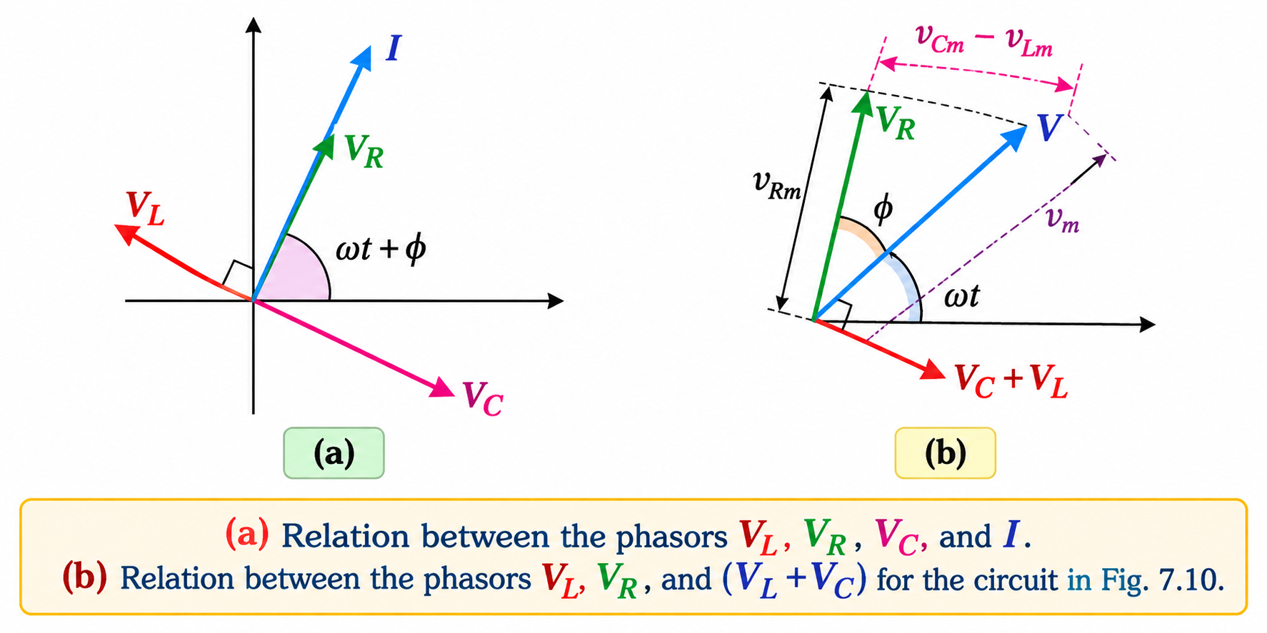
Let current phasor $\vec{I}$ be taken along the positive X-axis as reference.

Voltage across $R$: $\vec{V}_R = I R$ (along X-axis, in phase with $I$).
Voltage across $L$: $\vec{V}_L = I X_L$ (along +Y-axis, leads $I$ by $90^\circ$).
Voltage across $C$: $\vec{V}_C = I X_C$ (along -Y-axis, lags $I$ by $90^\circ$).

Dual-panel Phasor Relationship Diagram for Series LCR Circuit

Full Derivation: Impedance ($Z$) and Phase Angle ($\phi$) Assuming $V_L > V_C$ (Inductive Circuit), the net reactive voltage vector is $(V_L - V_C)$ pointing straight up along +Y-axis.
By Pythagorean theorem on the right-angled voltage triangle: $$V^2 = V_R^2 + (V_L - V_C)^2$$ Substitute $V = I Z$, $V_R = I R$, $V_L = I X_L$, and $V_C = I X_C$: $$\begin{aligned} (I Z)^2 &= (I R)^2 + (I X_L - I X_C)^2 \\ &= I^2 [ R^2 + (X_L - X_C)^2 ] \end{aligned}$$ Dividing both sides by $I^2$ and taking square root gives Impedance ($Z$): $$\mathbf{Z = \sqrt{R^2 + (X_L - X_C)^2} = \sqrt{R^2 + \left(\omega L - \frac{1}{\omega C}\right)^2}}$$ 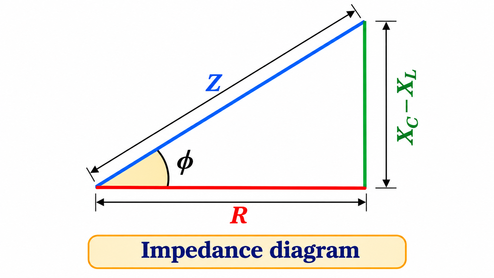From the Impedance Triangle, the phase angle $\phi$ between net voltage $V$ and current $I$ is: $$\mathbf{\tan\phi = \frac{X_L - X_C}{R} = \frac{\omega L - \frac{1}{\omega C}}{R}}$$

Phasor Diagram and Waveforms for Series LCR Circuit where XC > XL

Three Operating Regimes of Series LCR Circuit

Inductive Case ($X_L > X_C$): $\tan\phi > 0 \implies \phi$ is positive. Voltage leads current by phase angle $\phi$. Circuit behaves like an $R-L$ circuit.
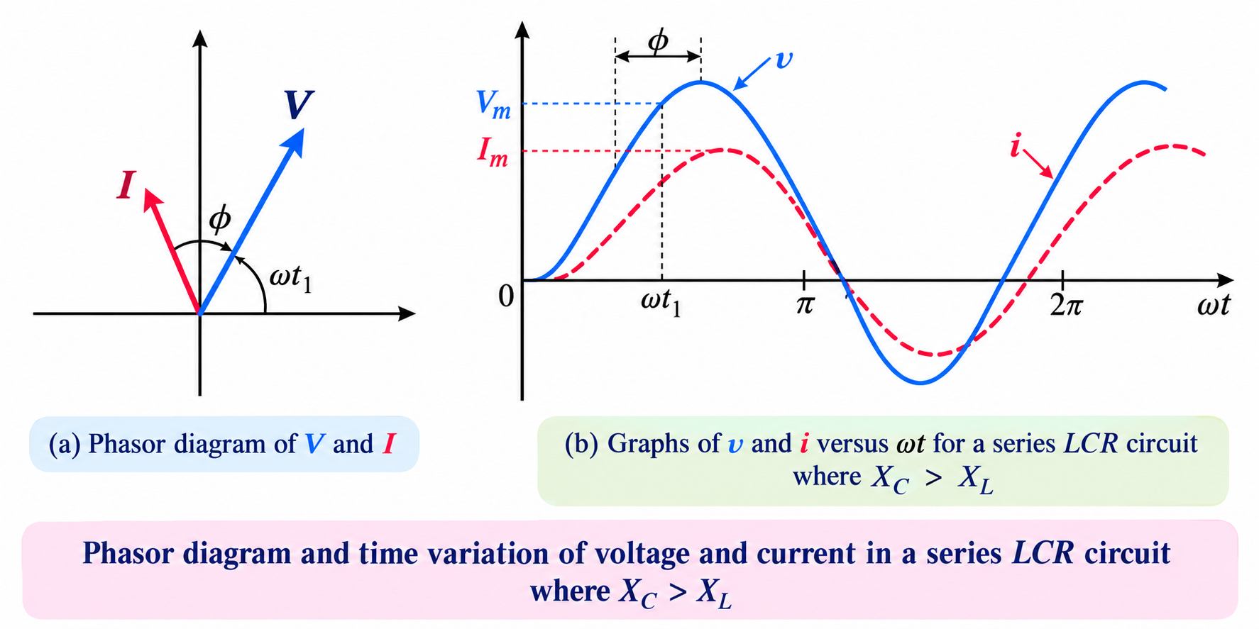
Capacitive Case ($X_C > X_L$): $\tan\phi < 0 \implies \phi$ is negative. Current leads voltage by phase angle $|\phi|$. Circuit behaves like an $R-C$ circuit.
Resistive Case ($X_L = X_C$): $\tan\phi = 0 \implies \phi = 0^\circ$. Voltage and current are perfectly in phase! Circuit is in Resonance.

B. Analytical Solution using Differential Equations (NCERT 7.6.2)

Applying Kirchhoff's Loop Rule to series LCR circuit:

$$v_L + v_C + v_R = v \implies L \frac{di}{dt} + \frac{q}{C} + i R = V_m \sin\omega t$$

Since $i = \frac{dq}{dt}$ and $\frac{di}{dt} = \frac{d^2q}{dt^2}$, we get the second-order differential equation:

$$\mathbf{L \frac{d^2q}{dt^2} + R \frac{dq}{dt} + \frac{q}{C} = V_m \sin\omega t}$$

Solving this gives steady-state charge $q = q_m \sin(\omega t + \theta)$ and current $i = \frac{dq}{dt} = I_m \sin(\omega t + \phi)$ where $I_m = \frac{V_m}{\sqrt{R^2 + (\omega L - 1/\omega C)^2}}$, proving identical results to the phasor method!

6. Resonance in Series LCR Circuit & Quality Factor (Q-factor)

Resonance: A series LCR circuit is said to be in resonance when the frequency of the applied AC source matches the natural frequency of the LC circuit, causing inductive reactance to cancel capacitive reactance ($X_L = X_C$), minimizing impedance to $Z = R$, and driving current amplitude to its absolute maximum!

Derivation: Resonant Frequency ($f_r$ or $\omega_r$) At resonance condition: $X_L = X_C$.
$$\omega_r L = \frac{1}{\omega_r C} \implies \omega_r^2 = \frac{1}{L C}$$ Taking square root gives Resonant Angular Frequency ($\omega_r$): $$\mathbf{\omega_r = \frac{1}{\sqrt{LC}} \quad \text{(Unit: rad/s)}}$$ Resonant Frequency in Hertz ($f_r$): $$\mathbf{f_r = \frac{\omega_r}{2\pi} = \frac{1}{2\pi\sqrt{LC}} \quad \text{(Unit: Hz)}}$$

Sharpness of Resonance & Quality Factor (Q-factor)

The Quality Factor (Q-factor) measures how sharp or narrow the resonance peak is. A high Q-factor means the circuit responds strongly to a very narrow band of frequencies (essential for radio and TV tuning selectivity!).

Full Derivation: Quality Factor ($Q$) Definition 1: Ratio of resonant frequency ($\omega_r$) to Bandwidth ($\Delta\omega = \omega_2 - \omega_1 = \frac{R}{L}$): $$Q = \frac{\omega_r}{2\Delta\omega} = \frac{\omega_r}{\left(\frac{R}{L}\right)} = \mathbf{\frac{\omega_r L}{R}}$$ Substitute $\omega_r = \frac{1}{\sqrt{LC}}$: $$Q = \frac{1}{\sqrt{LC}} \cdot \frac{L}{R} = \mathbf{\frac{1}{R} \sqrt{\frac{L}{C}}}$$ Definition 2 (Voltage Magnification): Ratio of voltage drop across Inductor ($V_L$) or Capacitor ($V_C$) to applied voltage across Resistor ($V_R$) at resonance: $$Q = \frac{V_L}{V_R} = \frac{I_m X_L}{I_m R} = \frac{\omega_r L}{R}$$

7. Power in AC Circuits, Power Factor & Wattless Current

Instantaneous power in an AC circuit is $p = v \cdot i = [V_m \sin\omega t] \cdot [I_m \sin(\omega t - \phi)]$.

Full Derivation: Average Power in AC Circuit Using trigonometric product formula $2\sin A \sin B = \cos(A-B) - \cos(A+B)$: $$\begin{aligned} p &= V_m I_m \sin\omega t \sin(\omega t - \phi) \\ &= \frac{V_m I_m}{2} [ \cos\phi - \cos(2\omega t - \phi) ] \end{aligned}$$ Average power over one complete cycle ($P_{\text{avg}}$): $$\begin{aligned} P_{\text{avg}} &= \frac{1}{T} \int_0^T p \, dt \\ &= \frac{V_m I_m}{2} \cos\phi - \frac{V_m I_m}{2} \frac{1}{T} \int_0^T \cos(2\omega t - \phi) \, dt \\ &= \frac{V_m I_m}{2} \cos\phi = \left(\frac{V_m}{\sqrt{2}}\right) \left(\frac{I_m}{\sqrt{2}}\right) \cos\phi \\ &= \mathbf{V_{\text{rms}} I_{\text{rms}} \cos\phi} \end{aligned}$$

Power Factor ($\cos\phi$) Power Factor is defined as the ratio of True Power ($P_{\text{avg}}$) to Apparent Power ($V_{\text{rms}} I_{\text{rms}}$): $$\mathbf{\text{Power Factor } (\cos\phi) = \frac{P_{\text{avg}}}{V_{\text{rms}} I_{\text{rms}}} = \frac{R}{Z} = \frac{R}{\sqrt{R^2 + (X_L - X_C)^2}}}$$

Pure Resistor / Resonance: $\phi = 0^\circ \implies \cos 0^\circ = 1$. Maximum power dissipation ($P_{\text{avg}} = V_{\text{rms}} I_{\text{rms}}$).
Pure Inductor / Pure Capacitor: $\phi = 90^\circ \implies \cos 90^\circ = 0$. Zero net power dissipation ($P_{\text{avg}} = 0$)!

Wattless Current (Idle Current)

In a purely inductive or capacitive circuit ($\phi = 90^\circ$), current flows through the circuit without consuming any average electric power. The component of RMS current perpendicular to voltage ($I_{\text{rms}} \sin\phi$) is called Wattless Current.

Application: Choke Coil A Choke Coil is a coil of very high self-inductance ($L$) and extremely low resistance ($R$) wound over a soft iron core. It is used to reduce AC current in tube lights / fluorescent lamps without significant power dissipation, since power factor $\cos\phi = \frac{R}{\sqrt{R^2 + \omega^2 L^2}} \approx 0$!

8. LC Oscillations

When a capacitor charged with initial charge $q_m$ is connected across an inductor of inductance $L$, electrical energy oscillates continuously back and forth between the electric field of the capacitor and the magnetic field of the inductor.

Full Derivation: LC Differential Equation & Energy Conservation By Kirchhoff's Loop Rule: $\frac{q}{C} + L \frac{di}{dt} = 0$.
Since $i = -\frac{dq}{dt}$ (current increases as charge decreases), $\frac{di}{dt} = -\frac{d^2q}{dt^2}$.
$$\frac{q}{C} - L \frac{d^2q}{dt^2} = 0 \implies \mathbf{\frac{d^2q}{dt^2} + \frac{1}{LC} q = 0}$$ This is identical to the simple harmonic motion (SHM) equation $\frac{d^2x}{dt^2} + \omega_0^2 x = 0$.
The natural frequency of LC oscillation is: $$\omega_0 = \frac{1}{\sqrt{LC}}$$ Solution for charge: $q(t) = q_m \cos(\omega_0 t)$.
Current: $i(t) = -\frac{dq}{dt} = q_m \omega_0 \sin(\omega_0 t) = I_m \sin(\omega_0 t)$.

Total Energy Conservation: $$\begin{aligned} U &= U_E + U_B = \frac{q^2}{2C} + \frac{1}{2} L i^2 \\ &= \frac{q_m^2 \cos^2\omega_0 t}{2C} + \frac{1}{2} L (q_m^2 \omega_0^2 \sin^2\omega_0 t) \\ &= \frac{q_m^2}{2C} [\cos^2\omega_0 t + \sin^2\omega_0 t] = \mathbf{\frac{q_m^2}{2C} = \text{Constant}} \end{aligned}$$

Electrical System (LC Circuit)	Mechanical System (Block on Spring)
Charge $q$	Displacement $x$
Current $i = \frac{dq}{dt}$	Velocity $v = \frac{dx}{dt}$
Inductance $L$	Mass $m$
Reciprocal Capacitance $1/C$	Spring Factor $k$
Electrical Energy $U_E = \frac{q^2}{2C}$	Potential Energy $U_P = \frac{1}{2} k x^2$
Magnetic Energy $U_B = \frac{1}{2} L i^2$	Kinetic Energy $U_K = \frac{1}{2} m v^2$

9. Transformers (Step-Up & Step-Down)

Definition: A static electrical device used to step up (increase) or step down (decrease) alternating voltage without changing frequency.

Operating Principle: Based on Mutual Induction. When alternating current flows through the primary coil, it sets up a changing magnetic flux in the soft iron core, which links with the secondary coil and induces an alternating EMF in it.

Full Derivation: Transformer Equation Let $\Phi$ be the magnetic flux linked per turn of core at time $t$.
Induced EMF in Primary Coil ($N_p$ turns): $v_p = -N_p \frac{d\Phi}{dt}$.
Induced EMF in Secondary Coil ($N_s$ turns): $v_s = -N_s \frac{d\Phi}{dt}$.
Dividing secondary EMF by primary EMF: $$\mathbf{\frac{v_s}{v_p} = \frac{N_s}{N_p} = k} \quad \text{(Transformation Ratio)}$$ For an ideal transformer (100% efficient, zero energy loss): $$\text{Input Power} = \text{Output Power} \implies v_p i_p = v_s i_s$$ $$\mathbf{\frac{i_p}{i_s} = \frac{v_s}{v_p} = \frac{N_s}{N_p} = k}$$

Parameter	Step-Up Transformer	Step-Down Transformer
Turn Ratio ($k$)	$k > 1 \implies N_s > N_p$	$k < 1 \implies N_s < N_p$
Voltage ($V$)	$V_s > V_p$ (Increases voltage)	$V_s < V_p$ (Decreases voltage)
Current ($I$)	$I_s < I_p$ (Decreases current)	$I_s > I_p$ (Increases current)
Winding Wires	Primary thick, Secondary thin	Primary thin, Secondary thick

Transformer Efficiency ($\eta$)

$$\eta = \frac{\text{Output Power}}{\text{Input Power}} \times 100\% = \frac{V_s I_s}{V_p I_p} \times 100\%$$

5 Major Energy Losses in Real Transformers & Mitigations (Board Favorite)

Copper Loss ($I^2R$ Heating): Current flowing through copper windings generates Joule heat. Mitigation: Use thick copper wires with low resistance.
Eddy Current (Iron) Loss: Alternating magnetic flux induces circulating eddy currents in the iron core, causing heating. Mitigation: Use a laminated soft iron core insulated with varnish.
Hysteresis Loss: Continuous magnetisation and demagnetisation of core every cycle consumes energy as heat. Mitigation: Core made of Soft Iron (small hysteresis loop area).
Flux Leakage: Not all magnetic flux generated by primary links with secondary. Mitigation: Wind primary and secondary coils directly over each other.
Humming Loss: Magnetostriction causes core to expand/contract, producing buzzing sound. Mitigation: Tightly clamp laminated core sheets.

10. High-Yield ICSE & CBSE Exam Practice Drills

Exam Drill 1 — Peak to RMS Values Question: An alternating voltage is described by $v = 282.8 \sin(314 t) \text{ V}$. Calculate: (i) Peak voltage, (ii) RMS voltage, (iii) Frequency of AC supply, and (iv) Instantaneous voltage at $t = 1/600 \text{ s}$.

Solution:
Comparing with $v = V_m \sin\omega t$:
(i) Peak Voltage $V_m = \mathbf{282.8 \text{ V}}$.
(ii) RMS Voltage $V_{\text{rms}} = \frac{V_m}{\sqrt{2}} = \frac{282.8}{1.414} = \mathbf{200 \text{ V}}$.
(iii) $\omega = 314 \text{ rad/s} \implies 2\pi f = 314 \implies f = \frac{314}{2 \times 3.14} = \mathbf{50 \text{ Hz}}$.
(iv) At $t = \frac{1}{600} \text{ s}$: $v = 282.8 \sin\left(314 \times \frac{1}{600}\right) = 282.8 \sin\left(\frac{\pi}{6}\right) = 282.8 \times 0.5 = \mathbf{141.4 \text{ V}}$.

Exam Drill 2 — Reactance of L & C Question: Find the reactance of a $10 \text{ mH}$ inductor and a $10 \text{ \mu F}$ capacitor at (a) DC ($0\text{ Hz}$), and (b) $50\text{ Hz}$ AC.

Solution:
(a) At DC ($f = 0$):
$X_L = 2\pi(0) L = \mathbf{0 \, \Omega}$ (Short circuit).
$X_C = \frac{1}{2\pi(0)C} = \mathbf{\infty \, \Omega}$ (Blocks DC completely).

(b) At $50\text{ Hz}$ AC ($f = 50$):
$X_L = 2\pi(50)(10 \times 10^{-3}) = 100\pi \times 10^{-2} = 3.14 \, \Omega$.
$X_C = \frac{1}{2\pi(50)(10 \times 10^{-6})} = \frac{1}{100\pi \times 10^{-6}} = \frac{10^4}{\pi} \approx \mathbf{318.3 \, \Omega}$.

Exam Drill 3 — Series LCR Complete Numerical Question: A series LCR circuit containing $R = 30 \, \Omega$, $L = 0.8 \text{ H}$, and $C = 50 \text{ \mu F}$ is connected across a $220\text{V}, 50\text{Hz}$ supply. Calculate: (i) Impedance $Z$, (ii) RMS Current $I_{\text{rms}}$, (iii) Phase Angle $\phi$, and (iv) Average Power Dissipated $P_{\text{avg}}$.

Solution:
Given: $V_{\text{rms}} = 220\text{V}, f = 50\text{Hz}, R = 30\,\Omega, L = 0.8\text{H}, C = 50\times 10^{-6}\text{F}$.
$X_L = 2\pi f L = 2 \times 3.14 \times 50 \times 0.8 = 251.2 \, \Omega$.
$X_C = \frac{1}{2\pi f C} = \frac{1}{2 \times 3.14 \times 50 \times 50 \times 10^{-6}} = \frac{10^6}{15700} = 63.7 \, \Omega$.
Net Reactance $(X_L - X_C) = 251.2 - 63.7 = 187.5 \, \Omega$.
(i) Impedance $Z = \sqrt{R^2 + (X_L - X_C)^2} = \sqrt{30^2 + (187.5)^2} = \sqrt{900 + 35156.25} = \mathbf{189.88 \, \Omega}$.
(ii) $I_{\text{rms}} = \frac{V_{\text{rms}}}{Z} = \frac{220}{189.88} = \mathbf{1.158 \text{ A}}$.
(iii) $\tan\phi = \frac{X_L - X_C}{R} = \frac{187.5}{30} = 6.25 \implies \phi \approx \mathbf{80.9^\circ}$ (Voltage leads current).
(iv) $P_{\text{avg}} = I_{\text{rms}}^2 R = (1.158)^2 \times 30 = \mathbf{40.23 \text{ W}}$.

Exam Drill 4 — Resonance & Q-Factor Question: A series LCR circuit has $L = 2.0\text{ H}, C = 32\text{ \mu F}, R = 10\,\Omega$. Calculate: (i) Resonant frequency $f_r$, and (ii) Q-factor of the circuit.

Solution:
(i) $\omega_r = \frac{1}{\sqrt{LC}} = \frac{1}{\sqrt{2.0 \times 32 \times 10^{-6}}} = \frac{1}{\sqrt{64 \times 10^{-6}}} = \frac{1}{8 \times 10^{-3}} = \mathbf{125 \text{ rad/s}}$.
$f_r = \frac{\omega_r}{2\pi} = \frac{125}{6.28} = \mathbf{19.9 \text{ Hz}}$.
(ii) $Q = \frac{\omega_r L}{R} = \frac{125 \times 2.0}{10} = \frac{250}{10} = \mathbf{25}$.

Exam Drill 5 — Transformer Efficiency Question: A step-down transformer operates on a $2200\text{V}$ line to supply $220\text{V}$ at $10\text{A}$ to a load. If its efficiency is $90\%$, find the current drawn from the primary line.

Solution:
Given: $V_p = 2200\text{V}, V_s = 220\text{V}, I_s = 10\text{A}, \eta = 90\% = 0.90$.
Output Power $P_s = V_s I_s = 220 \times 10 = 2200 \text{ W}$.
Since $\eta = \frac{P_s}{P_p} \implies P_p = \frac{P_s}{\eta} = \frac{2200}{0.90} = 2444.44 \text{ W}$.
$V_p I_p = 2444.44 \implies 2200 \times I_p = 2444.44 \implies I_p = \frac{2444.44}{2200} = \mathbf{1.11 \text{ A}}$.

11. Master Formula & Summary Comparison Table

Circuit Type	Opposition	Current Amplitude ($I_m$)	Phase Angle ($\phi$)	Power Factor ($\cos\phi$)	Average Power ($P_{\text{avg}}$)
Pure Resistor (R)	$R$	$I_m = \frac{V_m}{R}$	$\phi = 0^\circ$ (In Phase)	$1.0$ (Maximum)	$V_{\text{rms}} I_{\text{rms}}$
Pure Inductor (L)	$X_L = \omega L$ $= 2\pi f L$	$I_m = \frac{V_m}{X_L}$	$\phi = +90^\circ$ (I lags V)	$0.0$ (Zero)	$0$ (Wattless)
Pure Capacitor (C)	$X_C = \frac{1}{\omega C}$ $= \frac{1}{2\pi f C}$	$I_m = \frac{V_m}{X_C}$	$\phi = -90^\circ$ (I leads V)	$0.0$ (Zero)	$0$ (Wattless)
Series LCR Circuit	$Z = \sqrt{R^2 + (X_L - X_C)^2}$	$I_m = \frac{V_m}{Z}$	$\tan\phi = \frac{X_L - X_C}{R}$	$\frac{R}{Z}$	$V_{\text{rms}} I_{\text{rms}} \cos\phi$
LCR at Resonance	$Z_{\text{min}} = R$ ($X_L = X_C$)	$I_{\text{max}} = \frac{V_m}{R}$	$\phi = 0^\circ$ (In Phase)	$1.0$ (Maximum)	$V_{\text{rms}} I_{\text{rms}}$