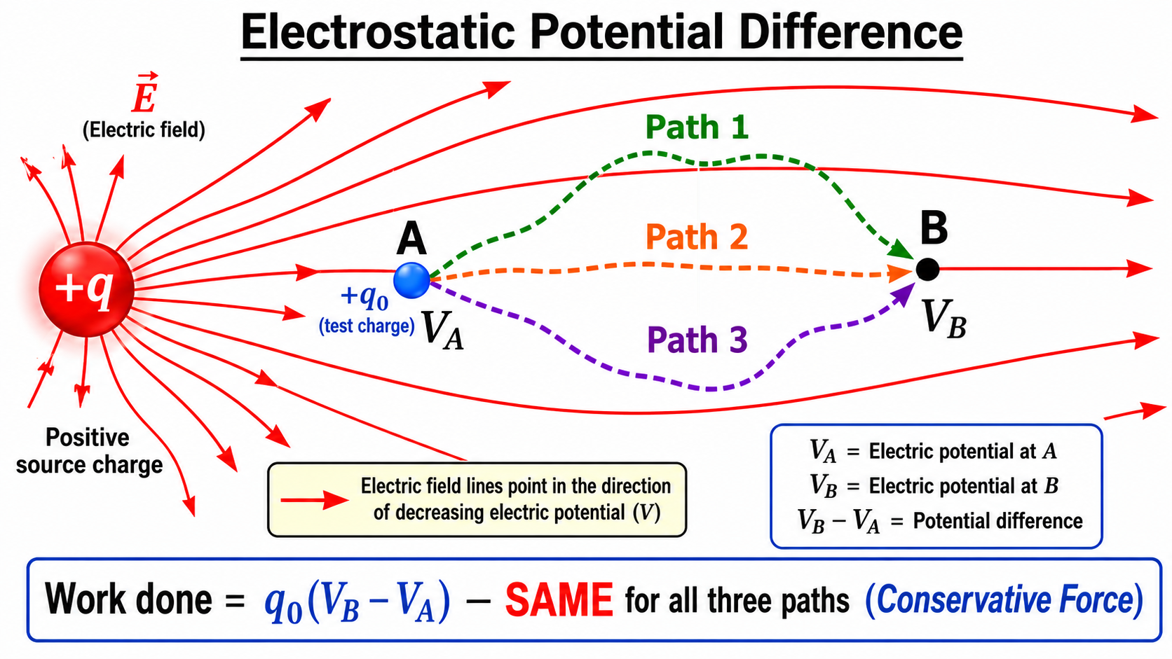
Let a source charge $+q$ be at origin O. We find the potential at point P, at a distance $r$ from O. We bring a test charge $+q_0$ from infinity to P very slowly (in equilibrium, no kinetic energy gained) along any path (say, radial).
At an intermediate distance $x$ from origin, the electrostatic (repulsive) force on the test charge is: $$\vec{F}_{elec} = \frac{1}{4\pi\epsilon_0} \frac{q \cdot q_0}{x^2} \hat{x} \quad \text{(directed away from O, i.e., outward)}$$
The external force required to move it without acceleration: $\vec{F}_{ext} = -\vec{F}_{elec}$ (directed inward).
Work done by external force from $\infty$ to $r$: $$W = \int_\infty^r \vec{F}_{ext} \cdot d\vec{x} = \int_\infty^r \left(-\frac{1}{4\pi\epsilon_0} \frac{q q_0}{x^2}\right)(-dx)$$ $$W = \frac{q q_0}{4\pi\epsilon_0} \int_\infty^r \frac{dx}{x^2}$$ $$= \frac{q q_0}{4\pi\epsilon_0}\left[-\frac{1}{x}\right]_\infty^r$$ $$= \frac{q q_0}{4\pi\epsilon_0}\left(-\frac{1}{r} + \frac{1}{\infty}\right) = \frac{q q_0}{4\pi\epsilon_0 r}$$
Since $V = \frac{W}{q_0}$, we get:
Since potential is a scalar quantity, the net potential at a point due to a system of $n$ charges is simply the algebraic sum of the individual potentials. No vector addition needed!
$$V_{net} = V_1 + V_2 + \cdots + V_n = \frac{1}{4\pi\epsilon_0}\sum_{i=1}^{n}\frac{q_i}{r_i}$$where $r_i$ is the distance of the $i$-th charge from the point in question, and $q_i$ carries its sign.
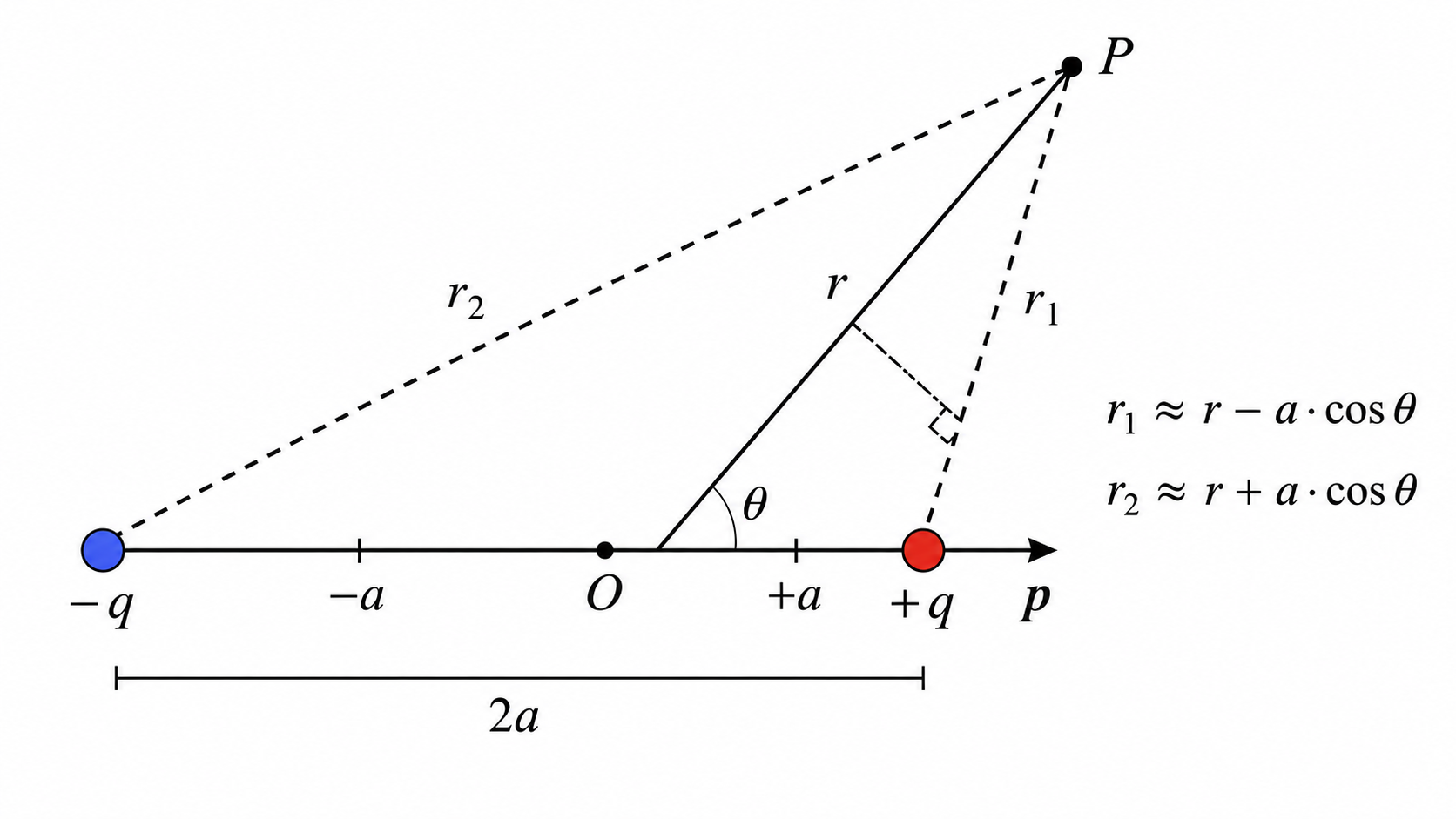
A dipole consists of two equal and opposite charges $+q$ and $-q$ separated by a small distance $2a$, with dipole moment $\vec{p} = q \times 2a$ directed from $-q$ to $+q$.
Let point P be at distance $r$ from the centre O of the dipole. Let OP make angle $\theta$ with the dipole axis (direction of $\vec{p}$). Let $r_1$ = distance from $+q$ to P, and $r_2$ = distance from $-q$ to P.
For a short dipole ($r \gg a$), using the perpendicular dropped from $+q$ and $-q$ to line OP:
Net potential at P: $$V = \frac{1}{4\pi\epsilon_0}\left[\frac{q}{r_1} + \frac{(-q)}{r_2}\right]$$ $$= \frac{q}{4\pi\epsilon_0}\left[\frac{1}{r-a\cos\theta} - \frac{1}{r+a\cos\theta}\right]$$ $$V = \frac{q}{4\pi\epsilon_0}\cdot\frac{(r+a\cos\theta)-(r-a\cos\theta)}{r^2-a^2\cos^2\theta}$$ $$= \frac{q}{4\pi\epsilon_0}\cdot\frac{2a\cos\theta}{r^2-a^2\cos^2\theta}$$
Since $r \gg a$, we have $r^2 \gg a^2\cos^2\theta$, so we drop $a^2\cos^2\theta$. Also $q \times 2a = p$:
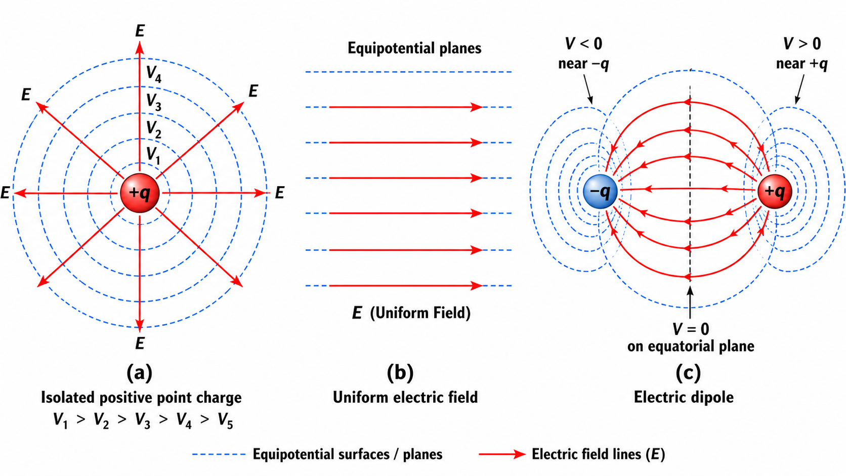
Definition: A surface (real or imaginary) on which the electric potential has the same value at every point is called an equipotential surface. Moving a charge along such a surface requires zero work since $\Delta V = 0$.
| Charge Configuration | Shape of Equipotential Surfaces | Shape of Field Lines |
|---|---|---|
| Isolated Positive Point Charge | Concentric spheres centred on the charge (closer near charge, farther away) | Radial straight lines pointing outward from the charge |
| Isolated Negative Point Charge | Concentric spheres centred on the charge | Radial straight lines pointing inward towards the charge |
| Uniform Electric Field (e.g., between large plates) | Flat planes perpendicular to the field direction (equally spaced) | Parallel straight lines (equally spaced) |
| Electric Dipole | Complex 3D surfaces — near each charge they look like spheres, but in between they form saddle-shaped surfaces | From $+q$ to $-q$, curving around; like loops of a bar magnet |
| Surface of a Conductor | The surface itself is equipotential; entire interior volume is also equipotential | Lines emerge perpendicular to the conductor surface |
Consider moving a unit positive charge through a small displacement $dr$ in the direction of field $\vec{E}$. The work done by the field: $dW = E\,dr$. By definition $dW = -dV$. Therefore:
$$\boxed{E = -\frac{dV}{dr}}$$The quantity $\frac{dV}{dr}$ is called the potential gradient. SI unit: V/m (same as N/C for electric field).
For $n$ charges, calculate the potential energy for every distinct pair and add algebraically. For $n$ charges, there are $\dfrac{n(n-1)}{2}$ pairs.
For three charges $q_1, q_2, q_3$ at mutual separations $r_{12}, r_{23}, r_{13}$:
$$\boxed{\begin{aligned} U &= \frac{1}{4\pi\epsilon_0} \Big[ \frac{q_1 q_2}{r_{12}} \\ & \quad + \frac{q_2 q_3}{r_{23}} + \frac{q_1 q_3}{r_{13}} \Big] \end{aligned}}$$If the external field creates a potential $V(\vec{r})$ at the position of charge $q$:
$$\boxed{U = qV(\vec{r})}$$Example: A charge $+Q$ placed at a point where external potential is $V_0$ has PE = $QV_0$. If $V_0 > 0$ and $Q > 0$, then $U > 0$ (energy was stored).
Consider two charges $q_1$ at $\vec{r_1}$ and $q_2$ at $\vec{r_2}$ in an external field that produces potentials $V(\vec{r_1})$ and $V(\vec{r_2})$ at their positions. The total PE has three contributions:
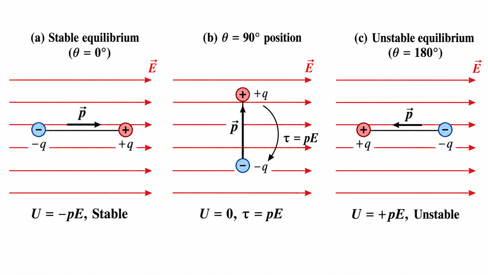
A dipole $\vec{p}$ placed in a uniform external field $\vec{E}$ at angle $\theta$ with the field experiences a torque that tends to align it. The torque magnitude: $\tau = pE\sin\theta$.
Work done by external torque to rotate dipole from angle $\theta_1$ to $\theta_2$: $$W = \int_{\theta_1}^{\theta_2}\tau\,d\theta = pE\int_{\theta_1}^{\theta_2}\sin\theta\,d\theta = pE[-\cos\theta]_{\theta_1}^{\theta_2} = pE(\cos\theta_1 - \cos\theta_2)$$
Taking $\theta_1 = 90°$ as the reference position ($U = 0$) and $\theta_2 = \theta$: $$W = pE(\cos90° - \cos\theta) = pE(0 - \cos\theta) = -pE\cos\theta$$ This work equals the potential energy stored:
| Orientation (θ) | PE (U) | Stability | Torque |
|---|---|---|---|
| $0^\circ$ (aligned with field) | $-pE$ (minimum) | Stable equilibrium | $0$ (no tendency to rotate) |
| $90^\circ$ (perpendicular) | $0$ (reference) | Neither stable nor unstable | $pE$ (maximum) |
| $180^\circ$ (anti-parallel) | $+pE$ (maximum) | Unstable equilibrium | $0$ (but any small displacement rotates it) |
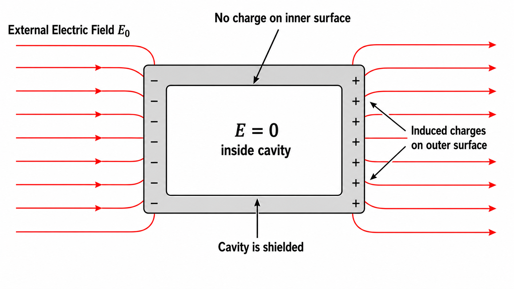
The interior cavity of a hollow conductor is completely shielded from external electric fields.
Applications:
| Property | Non-polar Molecules | Polar Molecules |
|---|---|---|
| Centre of positive charge | Coincides with centre of negative charge | Does NOT coincide with centre of negative charge |
| Net dipole moment (without field) | Zero | Non-zero (permanent dipole moment) |
| Examples | H₂, O₂, N₂, CO₂, CH₄, C₆H₆ | H₂O, HCl, NH₃, SO₂, HF |
| Behaviour in external field | Field induces a dipole moment (stretches the electron cloud) | Field partially aligns the permanent dipoles |
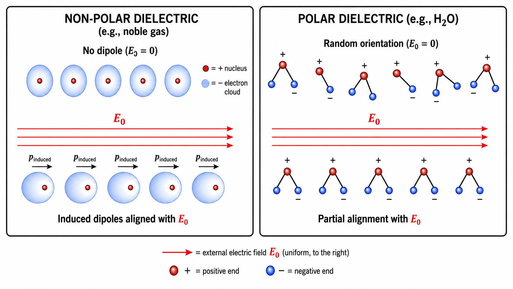
When a dielectric is placed in an external electric field $\vec{E}_0$:
In both cases, the net effect is: the dielectric develops a macroscopic dipole moment per unit volume, called the Polarisation Vector $\vec{P}$.
| Material | Dielectric Constant (K) | Electric Susceptibility ($\chi_e = K - 1$) |
|---|---|---|
| Vacuum | 1 (definition) | 0 |
| Air (dry) | ≈ 1.0006 | ≈ 0.0006 |
| Paraffin | 2.2 | 1.2 |
| Paper | 3.5 | 2.5 |
| Mica | 5–7 | 4–6 |
| Glass | 5–10 | 4–9 |
| Water (liquid) | 80 | 79 |
| Titanate ceramics | ~10,000 | ~9,999 |
When charge $+Q$ is given to one plate, it induces charge $-Q$ on the other plate (connected to ground or being a conductor). This creates a potential difference $V$ between the plates.
A parallel plate capacitor consists of two large, flat, parallel conducting plates each of area $A$, separated by distance $d$, with $d \ll \sqrt{A}$ (edge effects negligible). Plate 1 carries $+Q$ (surface charge density $\sigma = Q/A$), Plate 2 carries $-Q$.
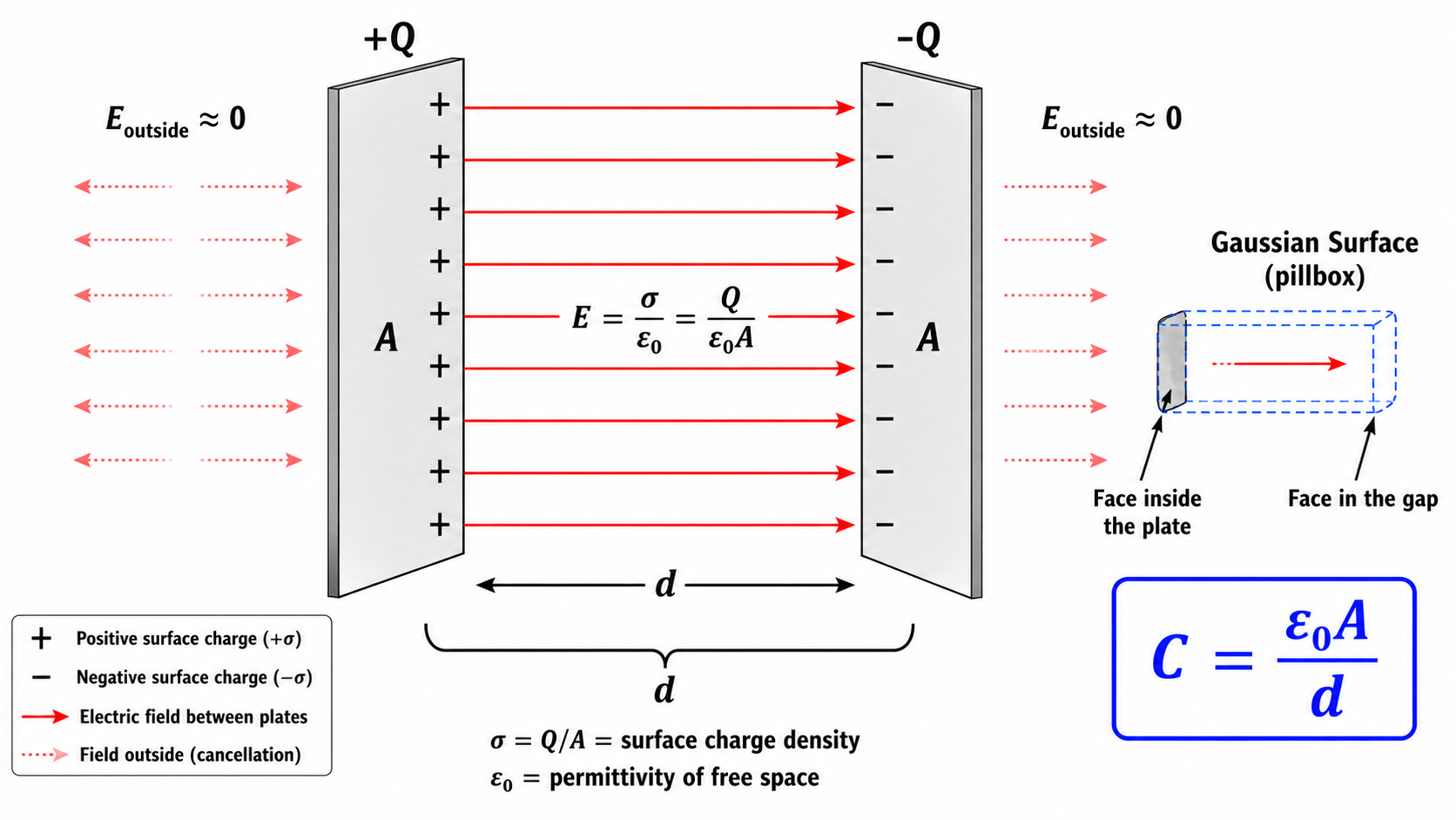
Step 1: Find Electric Field between the plates.
Each plate acts as an infinite plane of charge. Using Gauss's Law (pillbox Gaussian surface):
$$E_{each\,plate} = \frac{\sigma}{2\epsilon_0}$$
Between the plates, fields from both plates add up (same direction):
$$\boxed{E = \frac{\sigma}{\epsilon_0} = \frac{Q}{\epsilon_0 A}} \quad \text{(uniform, from + to − plate)}$$
Outside the capacitor, fields from both plates cancel: $E_{outside} = 0$.
Step 2: Find Potential Difference $V$ between the plates.
In a uniform field, potential difference = field × distance:
$$V = E \times d = \frac{Qd}{\epsilon_0 A}$$
Step 3: Calculate Capacitance. $$C = \frac{Q}{V} = \frac{Q}{\dfrac{Qd}{\epsilon_0 A}}$$
When a capacitor is charged from $q=0$ to $q=Q$, at an intermediate stage when charge is $q$ and potential is $v = q/C$, the work done in adding a further small charge $dq$: $$dW = v\,dq = \frac{q}{C}\,dq$$ Total work done (= energy stored) in charging from 0 to $Q$: $$U = \int_0^Q \frac{q}{C}\,dq = \frac{1}{C}\cdot\frac{q^2}{2}\bigg|_0^Q = \frac{Q^2}{2C}$$
All three forms are equivalent (use $Q = CV$ to convert between them). Choose the most convenient form depending on what is given.
Energy Density (Energy per unit volume of field): $$\boxed{u = \frac{U}{\text{Volume}} = \frac{\frac{1}{2}CV^2}{Ad} = \frac{\frac{1}{2}\cdot\frac{\epsilon_0 A}{d}\cdot(Ed)^2}{Ad} = \frac{1}{2}\epsilon_0 E^2}$$ This is a universal formula — energy density of any electric field is $\dfrac{1}{2}\epsilon_0 E^2$.
When the full space between the plates is filled with a dielectric of constant $K$:
where $\epsilon_r = K$ is the relative permittivity and $\epsilon = K\epsilon_0$ is the absolute permittivity of the dielectric.
A dielectric slab of thickness $t$ (where $t < d$) and dielectric constant $K$ is inserted between the plates. The remaining gap $(d - t)$ is vacuum.
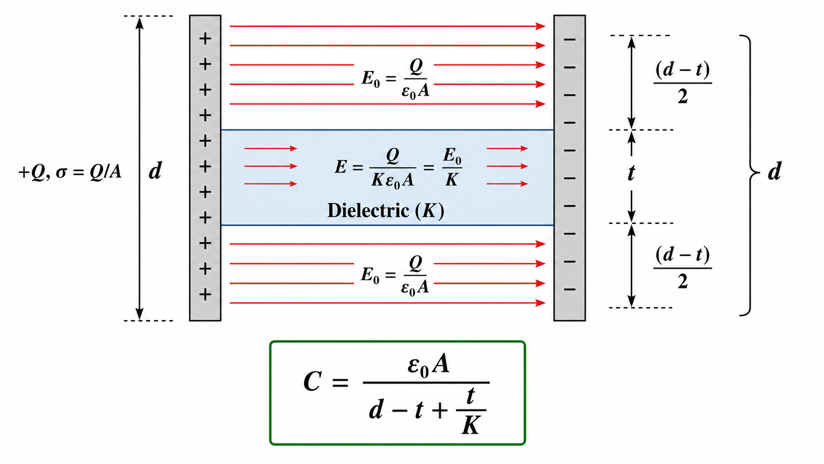
Step 1: Electric field in each region.
The surface charge density $\sigma = Q/A$ is unchanged. Using boundary conditions (normal D-field is continuous):
$$E_0 = \frac{Q}{\epsilon_0 A} \quad \text{(vacuum region of thickness } d-t\text{)}$$
$$E = \frac{Q}{K\epsilon_0 A} = \frac{E_0}{K} \quad \text{(inside dielectric of thickness } t\text{)}$$
Step 2: Total potential difference $V$. $$V = E_0(d-t) + E \cdot t$$ $$= \frac{Q}{\epsilon_0 A}(d-t) + \frac{Q}{K\epsilon_0 A}\cdot t$$ $$= \frac{Q}{\epsilon_0 A}\left[(d-t) + \frac{t}{K}\right]$$
Step 3: Capacitance $C = Q/V$.
Special Cases:
• If $K \to \infty$ (conducting slab, not a dielectric but useful limit): $C = \dfrac{\epsilon_0 A}{d - t}$ — equivalent to reducing plate separation by $t$.
• If $K = 1$ (vacuum/air slab): $C = \dfrac{\epsilon_0 A}{d}$ — original capacitance (as expected).
• If $t = d$ (full dielectric): $C = \dfrac{K\epsilon_0 A}{d}$ — full dielectric formula.
When a dielectric slab (constant $K$) is inserted into a charged parallel plate capacitor, the outcome depends on whether the battery is connected:
| Quantity | Battery DISCONNECTED (Q = constant) | Battery CONNECTED (V = constant) |
|---|---|---|
| Capacitance $C$ | Increases: $C' = KC_0$ | Increases: $C' = KC_0$ |
| Charge $Q$ | Constant: $Q' = Q_0$ | Increases: $Q' = KQ_0$ (battery supplies more charge) |
| Voltage $V$ | Decreases: $V' = V_0/K$ | Constant: $V' = V_0$ (maintained by battery) |
| Electric Field $E$ | Decreases: $E' = E_0/K$ | Constant: $E' = E_0$ (same since $V, d$ unchanged) |
| Energy $U$ | Decreases: $U' = U_0/K$ (dielectric is pulled in — does work) | Increases: $U' = KU_0$ (battery does extra work; energy stored increases) |
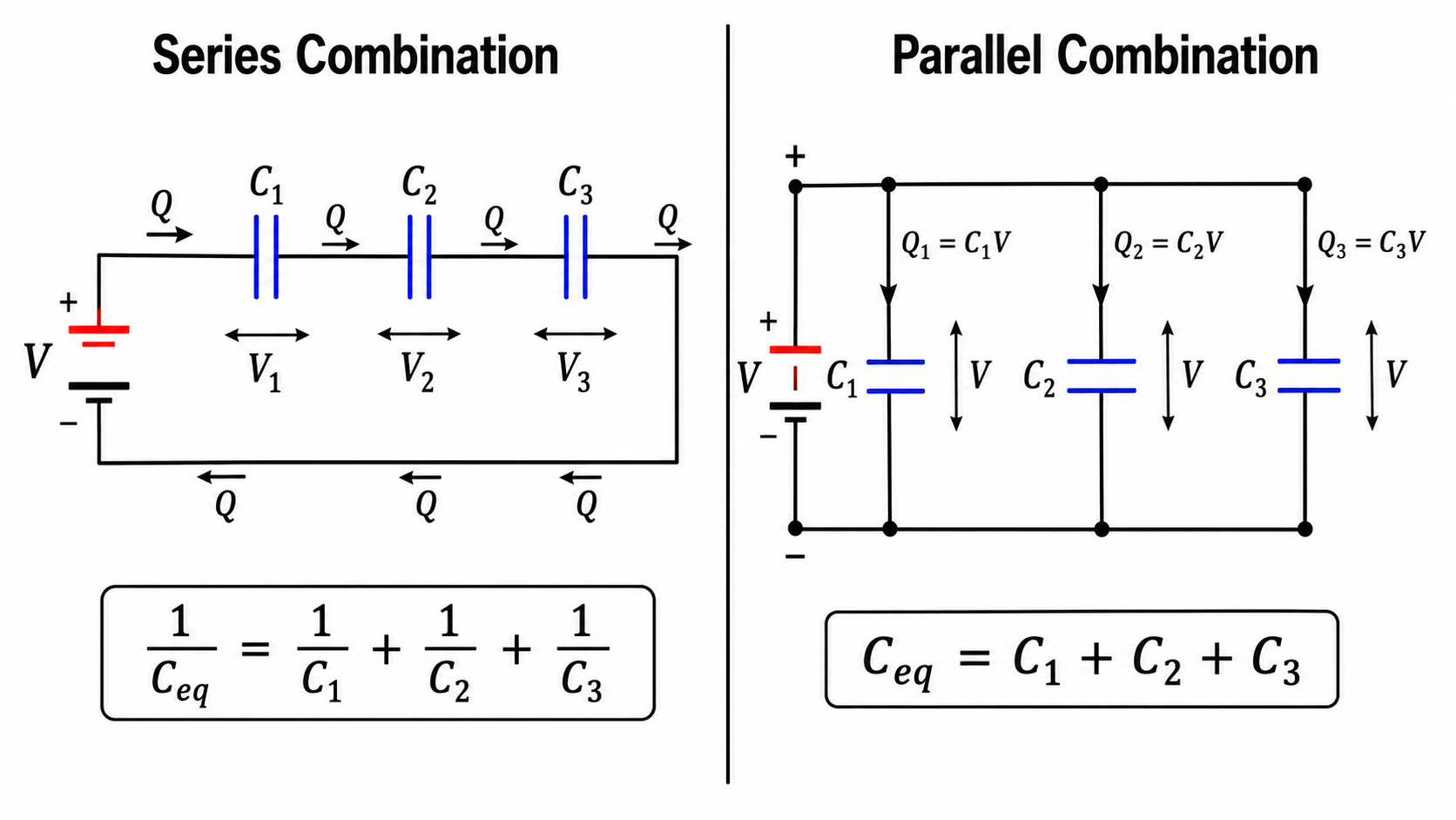
When capacitors are connected end-to-end (in a single chain), they are in series.
Key property of series: Same charge $Q$ appears on every capacitor (charge cannot accumulate between the capacitors in the chain). The total voltage splits.
For $n$ capacitors $C_1, C_2, \ldots, C_n$ in series with total voltage $V$: $$V = V_1 + V_2 + \cdots + V_n = \frac{Q}{C_1} + \frac{Q}{C_2} + \cdots + \frac{Q}{C_n} = Q\left(\frac{1}{C_1} + \frac{1}{C_2} + \cdots + \frac{1}{C_n}\right)$$ Since $V = Q/C_{eq}$, dividing both sides by $Q$:
For two capacitors in series: $C_{eq} = \dfrac{C_1 C_2}{C_1 + C_2}$ (product over sum).
Key property of parallel: Same voltage $V$ appears across every capacitor. The total charge splits.
For $n$ capacitors $C_1, C_2, \ldots, C_n$ in parallel with voltage $V$: $$Q = Q_1 + Q_2 + \cdots + Q_n = C_1V + C_2V + \cdots + C_nV = V(C_1 + C_2 + \cdots + C_n)$$ Since $Q = C_{eq}V$, dividing by $V$:
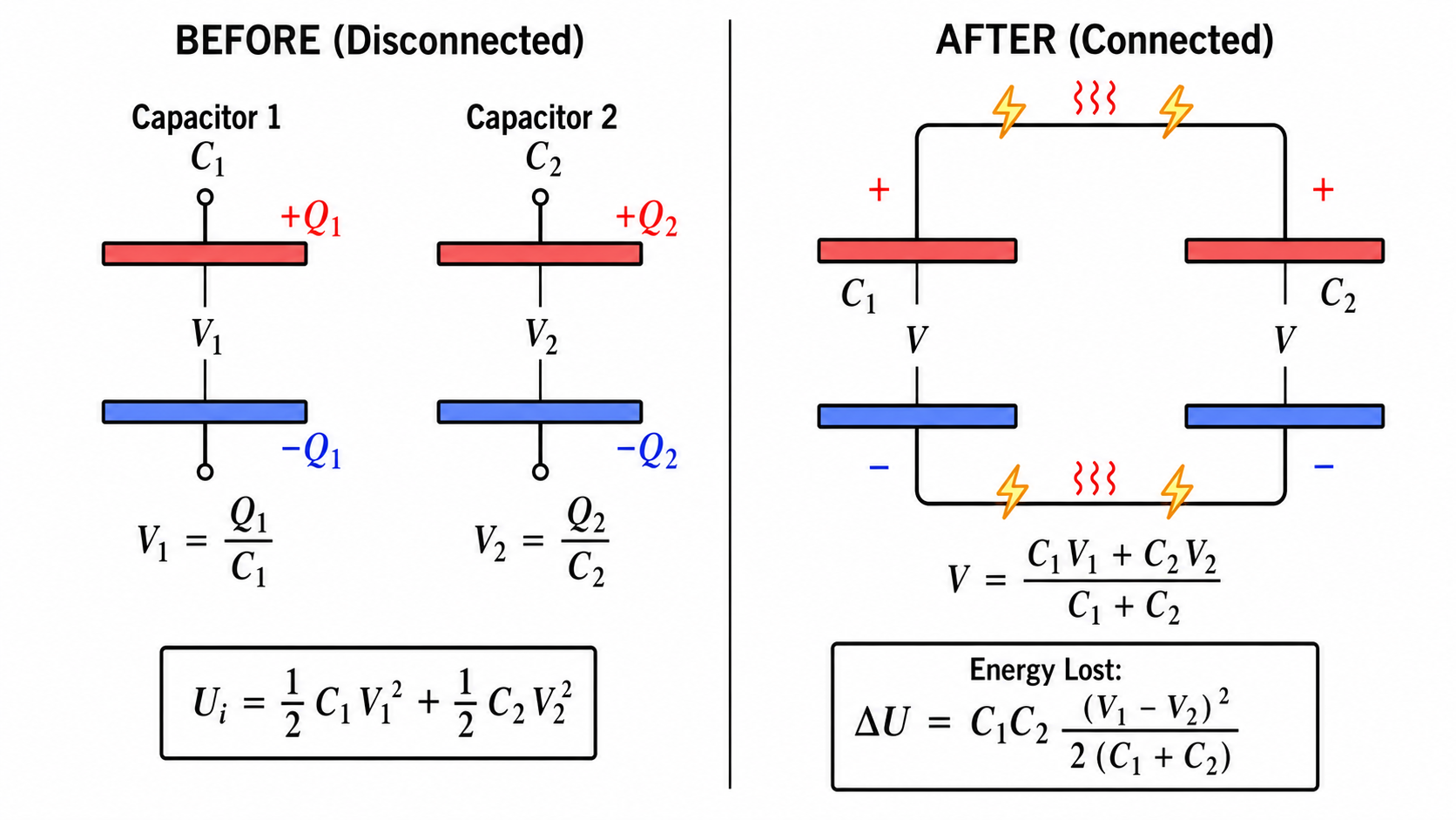
Let capacitor $C_1$ have initial charge $Q_1$ (at potential $V_1 = Q_1/C_1$), and capacitor $C_2$ have initial charge $Q_2$ (at potential $V_2 = Q_2/C_2$). They are connected positive plate to positive plate and negative plate to negative plate.
Principle of Conservation of Charge: Total charge is conserved (no charge is created or destroyed).
Total charge: $Q_{total} = Q_1 + Q_2$. After connection, both capacitors reach common potential $V_{common}$. New charges: $Q_1' = C_1 V$ and $Q_2' = C_2 V$. By conservation:
$$Q_1' + Q_2' = Q_1 + Q_2 \Rightarrow (C_1 + C_2)V = Q_1 + Q_2$$Initial total energy (before connection): $$U_i = \frac{1}{2}C_1 V_1^2 + \frac{1}{2}C_2 V_2^2$$
Final total energy (after connection, both at common potential $V$):
$$U_f = \frac{1}{2}(C_1 + C_2)V^2$$
$$= \frac{1}{2}(C_1+C_2)\left(\frac{C_1V_1+C_2V_2}{C_1+C_2}\right)^2$$
$$= \frac{(C_1V_1+C_2V_2)^2}{2(C_1+C_2)}$$
Energy lost:
$$\Delta U = U_i - U_f$$
$$= \frac{1}{2}C_1V_1^2 + \frac{1}{2}C_2V_2^2 - \frac{(C_1V_1+C_2V_2)^2}{2(C_1+C_2)}$$
After algebraic simplification (multiplying and expanding):
$$\Delta U = \frac{1}{2(C_1+C_2)}\Big[C_1(C_1+C_2)V_1^2$$
$$+ C_2(C_1+C_2)V_2^2 - (C_1V_1+C_2V_2)^2\Big]$$
$$\begin{aligned} &= \frac{1}{2(C_1+C_2)}\Big[C_1C_2V_1^2 \\ & \quad + C_1C_2V_2^2 - 2C_1C_2V_1V_2\Big] \end{aligned}$$