Chapter 1: Electric Charges and Fields

Welcome to Class 12 Physics! This opening chapter lays the foundation for all of Electromagnetism. The concepts of Coulomb's Law, Electric Fields, and Gauss's Law are not just crucial for your CBSE Board Exams (expecting at least one 5-marker derivation from here), but they also form a significant chunk of JEE Mains and Advanced mechanics-linked problems. Let's master the fundamentals.

1. Electric Charge and its Properties

Electric Charge ($q$ or $Q$) is an intrinsic property of elementary particles of matter which gives rise to electric force between various objects. It is a scalar quantity.

SI Unit: Coulomb ($C$). One Coulomb is defined as the amount of charge that flows through a cross-section of a wire in 1 second if there is a steady current of 1 Ampere ($1\text{C} = 1\text{A} \times 1\text{s}$).
Dimensional Formula: Since $I = q/t$, we have $[q] = [A \cdot T]$.
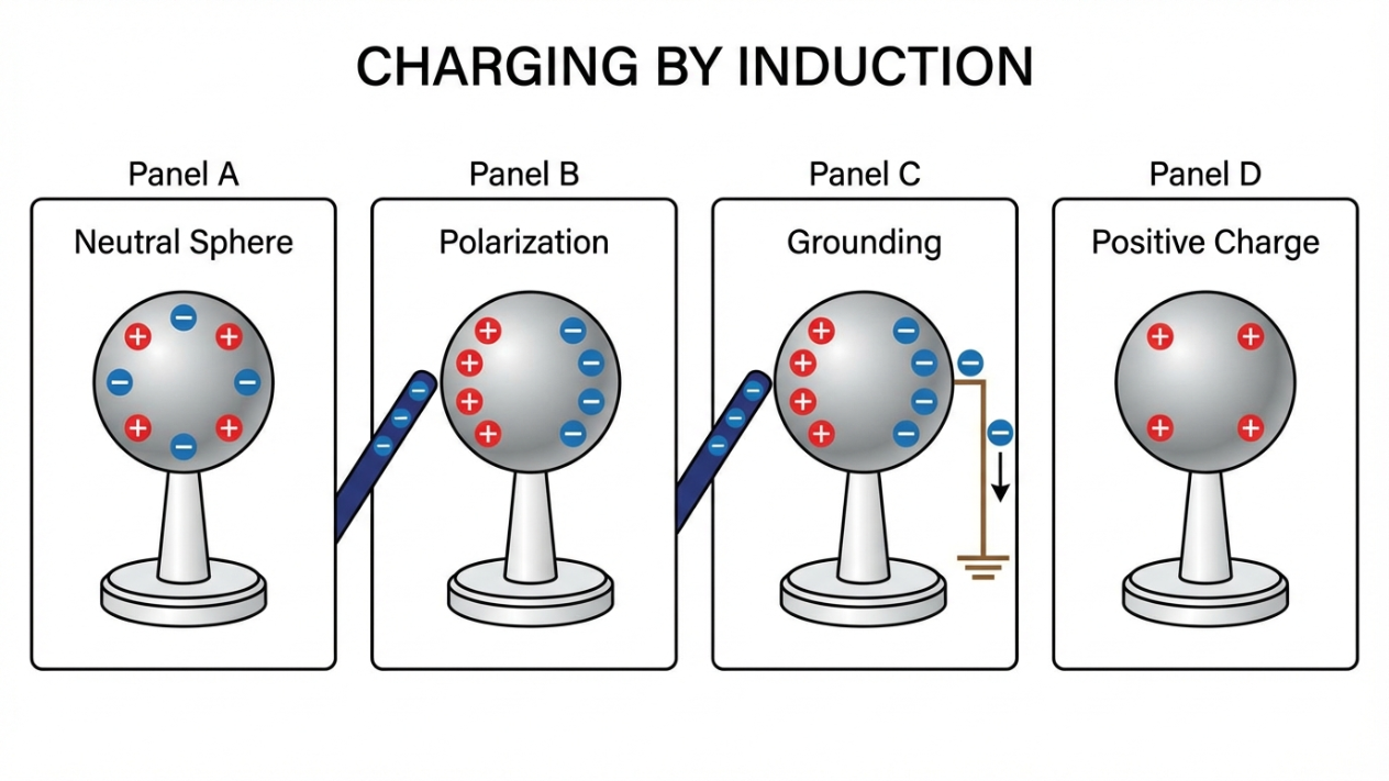
Types of Charges: Positive (e.g., protons, glass rod rubbed with silk) and Negative (e.g., electrons, plastic rod rubbed with wool). Like charges repel, unlike charges attract.

Basic Properties of Electric Charge (Crucial for Boards)

The 3 Core Properties

Additivity of Charges: The total charge of a system is the algebraic sum (including signs) of all individual charges in the system. ($Q_{net} = q_1 + q_2 + \dots + q_n$).
Conservation of Charge: The total charge of an isolated system remains constant. Charge can neither be created nor destroyed, only transferred from one body to another.
Quantization of Charge: The charge on any body is always an integral multiple of the basic quantum of charge ($e$), which is the charge on an electron. $$q = \pm ne$$ (where $n = 1, 2, 3\dots$ and $e = 1.6 \times 10^{-19} \text{ C}$)

Macroscopic vs. Microscopic Quantization: At the microscopic level (dealing with tens or hundreds of electrons), quantization is highly noticeable. However, at the macroscopic level (dealing with micro-coulombs $\mu C$), the number of electrons is so massive ($~10^{13}$) that the "grainy" nature of charge is lost, and charge appears to be continuous. Thus, quantization is often ignored at macroscopic scales.

JEE Main Transition: Mass Change Charging is solely the transfer of electrons. Since electrons have mass ($m_e = 9.1 \times 10^{-31} \text{ kg}$), charging affects the mass of a body slightly!
- A body that becomes positively charged has lost electrons, so its mass decreases.
- A body that becomes negatively charged has gained electrons, so its mass increases.
$\Delta m = n \times m_e$

Practice Problem 1 Question: How many electrons must be removed from a neutral body to give it a charge of $+1 \text{ C}$?

Solution:
Using Quantization of charge: $q = ne$
Given $q = 1 \text{ C}$ and $e = 1.6 \times 10^{-19} \text{ C}$.
$n = \frac{q}{e} = \frac{1}{1.6 \times 10^{-19}}$
$n = \frac{10}{16} \times 10^{19} = 0.625 \times 10^{19} = \mathbf{6.25 \times 10^{18} \text{ electrons}}$.

2. Coulomb's Law

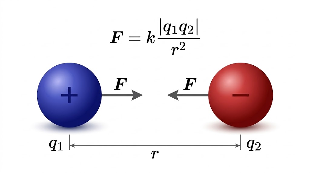
It states that the electrostatic force of attraction or repulsion between two stationary point charges is directly proportional to the product of the magnitudes of the charges and inversely proportional to the square of the distance between them.

Formula $$F = \frac{1}{4\pi\epsilon_0} \frac{|q_1| |q_2|}{r^2}$$

$\epsilon_0$ is the Permittivity of Free Space (Vacuum).
Value of $\epsilon_0 = 8.854 \times 10^{-12} \text{ C}^2/\text{N}\cdot\text{m}^2$.
Value of $\frac{1}{4\pi\epsilon_0} = 9 \times 10^9 \text{ N}\cdot\text{m}^2/\text{C}^2$.

Limitations of Coulomb's Law:
1. It is only valid for point charges (sizes of bodies are negligible compared to distance).
2. It is only valid for charges at rest (static). Moving charges also create magnetic fields.

Coulomb's Law in Vector Form (Board Derivation)

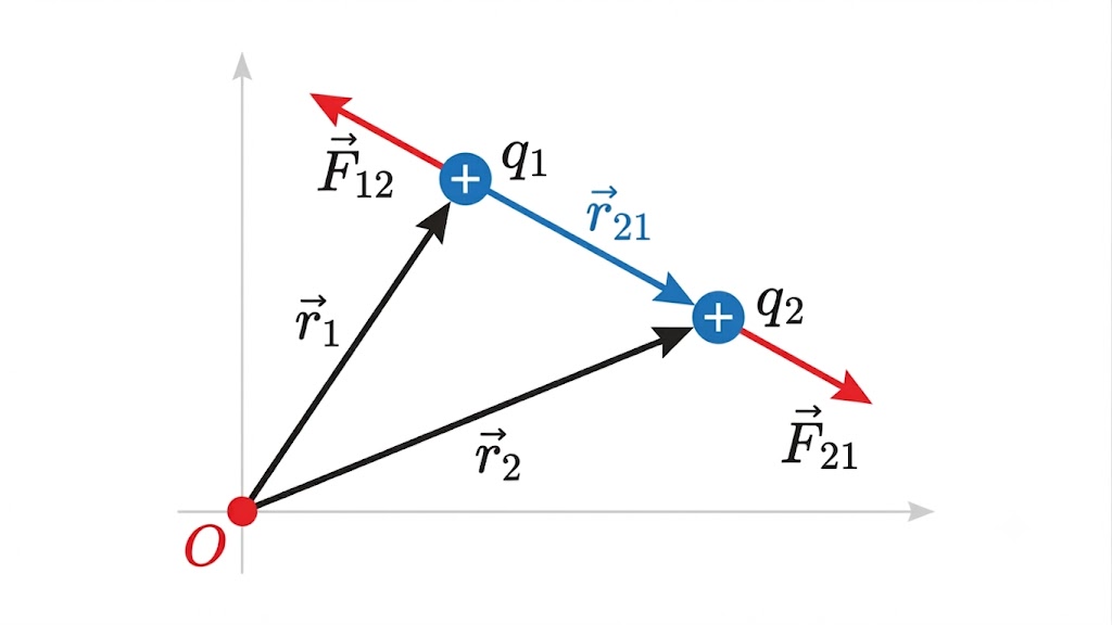
Let two point charges $q_1$ and $q_2$ be placed at position vectors $\vec{r}_1$ and $\vec{r}_2$ respectively.

The vector from $q_1$ to $q_2$ is $\vec{r}_{21} = \vec{r}_2 - \vec{r}_1$. The unit vector is $\hat{r}_{21} = \frac{\vec{r}_{21}}{|\vec{r}_{21}|}$.
The force exerted ON $q_2$ BY $q_1$ is $\vec{F}_{21}$:

$$\vec{F}_{21} = \frac{1}{4\pi\epsilon_0} \frac{q_1 q_2}{|\vec{r}_{21}|^2} \hat{r}_{21}$$

Similarly, the force exerted ON $q_1$ BY $q_2$ is $\vec{F}_{12}$:

$$\vec{F}_{12} = \frac{1}{4\pi\epsilon_0} \frac{q_1 q_2}{|\vec{r}_{12}|^2} \hat{r}_{12}$$

Since the unit vectors point in opposite directions ($\hat{r}_{12} = -\hat{r}_{21}$), we conclude:
$\vec{F}_{12} = -\vec{F}_{21}$.
Conclusion: Electrostatic forces obey Newton's Third Law of Motion (Action-Reaction pair).

Relative Permittivity / Dielectric Constant ($K$ or $\epsilon_r$)

When charges are placed in a medium other than vacuum, the force between them decreases because the medium gets polarized and creates an opposing field. The Permittivity of the medium ($\epsilon$) replaces $\epsilon_0$.

$$K = \epsilon_r = \frac{\epsilon}{\epsilon_0} = \frac{F_{vacuum}}{F_{medium}}$$

Therefore, $F_{medium} = \frac{F_{vacuum}}{K}$. (For water, $K \approx 81$, so electrostatic force drops 81 times in water!).

Principle of Superposition

The total force on any charge due to a number of other charges is the vector sum of all the individual forces acting on that charge. The individual forces are unaffected by the presence of other charges.

$$\vec{F}_{net} = \vec{F}_1 + \vec{F}_2 + \vec{F}_3 + \dots$$

JEE Main Transition: Equilibrium & SHM 1. Equilibrium of 3 Charges: If two charges $Q$ and $q$ are placed at a distance $L$, a third charge $q_0$ will be in equilibrium if placed between them such that the net force on it is zero.
If both $Q$ and $q$ are like charges, the null point is between them. Distance from $q$ (smaller charge) = $\frac{L}{\sqrt{Q/q} + 1}$.

2. SHM of a Charge: If a charge $+q_0$ is placed exactly midway between two $+Q$ charges and is slightly displaced along the line joining them, it experiences a restoring force and executes Simple Harmonic Motion (SHM). Time period $T = 2\pi \sqrt{\frac{m}{k_{SHM}}}$.

Practice Problem 2 Question: Two point charges $+4e$ and $+e$ are fixed a distance 'a' apart. Where should a third point charge $q$ be placed on the line joining the two charges so that it may be in equilibrium?

Solution:
Let the third charge $q$ be placed at a distance $x$ from $+e$ (smaller charge).
The distance from $+4e$ will be $(a - x)$.
For equilibrium, Force on $q$ due to $+e$ = Force on $q$ due to $+4e$.
$\frac{1}{4\pi\epsilon_0} \frac{q \cdot e}{x^2} = \frac{1}{4\pi\epsilon_0} \frac{q \cdot 4e}{(a-x)^2}$
Canceling common terms: $\frac{1}{x^2} = \frac{4}{(a-x)^2}$
Taking the square root on both sides (ignoring negative since it must be between them):
$\frac{1}{x} = \frac{2}{a-x}$
$a - x = 2x \implies 3x = a \implies \mathbf{x = \frac{a}{3}}$.
The charge must be placed at a distance of $a/3$ from the $+e$ charge.

3. Electric Field

An electric field is the space around a charge in which its electrostatic force can be experienced by another test charge.

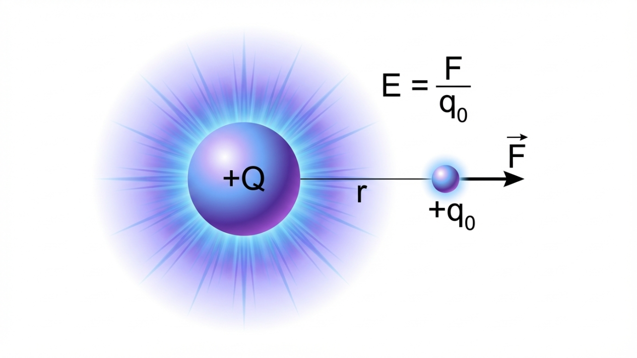
Definition & Formula Electric Field Intensity ($\vec{E}$) at a point is the force experienced by a vanishingly small positive test charge ($q_0$) placed at that point. $$\vec{E} = \lim_{q_0 \to 0} \frac{\vec{F}}{q_0}$$

SI Unit: Newton/Coulomb ($N/C$) or Volt/meter ($V/m$).
Dimensions: Force/Charge = $[MLT^{-2}] / [AT] = \mathbf{[MLT^{-3}A^{-1}]}$.
Direction: The direction of $\vec{E}$ is the direction of the force on a positive test charge. Therefore, it points away from positive charges and towards negative charges.

Electric Field due to a Point Charge

Let a source charge $+q$ be at the origin. A test charge $+q_0$ is placed at distance $r$.
Force $F = \frac{1}{4\pi\epsilon_0} \frac{q q_0}{r^2}$.
Since $E = F/q_0$, we get:

$$E = \frac{1}{4\pi\epsilon_0} \frac{q}{r^2}$$

In vector form: $\vec{E} = \frac{1}{4\pi\epsilon_0} \frac{q}{r^2} \hat{r}$. Notice that $E \propto 1/r^2$ (Inverse square law).

Electric Field due to a System of Charges (Superposition)

Just like force, the net electric field at a point due to multiple discrete charges is the vector sum of individual fields:
$\vec{E}_{net} = \vec{E}_1 + \vec{E}_2 + \dots + \vec{E}_n = \frac{1}{4\pi\epsilon_0} \sum_{i=1}^{n} \frac{q_i}{r_i^2} \hat{r}_i$

JEE Main Transition: Kinematics of Charged Particle When a particle of mass $m$ and charge $q$ is placed in a uniform electric field $E$, it experiences a constant force $F = qE$.
Acceleration of the particle: $a = \frac{qE}{m}$.
If a charge enters perpendicular to a uniform electric field with velocity $v$, it follows a parabolic trajectory. The vertical deflection after traveling a horizontal distance $x$ is: $y = \frac{qE}{2mv^2}x^2$.

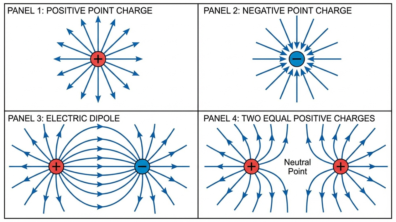
4. Electric Field Lines

Introduced by Michael Faraday, these are imaginary curves drawn in an electric field such that the tangent to the curve at any point gives the direction of the net electric field at that point.

Properties of Electric Field Lines (Direct Board 3-Marker)

They start from positive charges and end at negative charges. For a single charge, they may start or end at infinity.
Two field lines can NEVER intersect each other. Reason: The tangent to a field line gives the direction of the net electric field. If they did intersect, there would be two distinct tangents at the point of intersection, implying two different directions of the net electric field at a single point, which is logically and physically impossible.
They form continuous curves without any breaks in a charge-free region.
They do not form closed loops (due to the conservative nature of the electrostatic field).
The relative closeness of the lines indicates the strength of the electric field. (Crowded = strong field; Far apart = weak field).
Crucial: They are always normal (perpendicular) to the surface of a charged conductor, and the electric field inside a conductor is always zero.

5. Electric Dipole

An electric dipole is a system of two equal and opposite point charges ($+q$ and $-q$) separated by a small vector distance ($2\vec{a}$).

Electric Dipole Moment ($\vec{p}$): It measures the strength of the dipole.
$$\vec{p} = q \times 2\vec{a}$$
It is a vector quantity. Its direction is by convention from the negative charge to the positive charge. SI unit is Coulomb-meter ($C \cdot m$).

Electric Field due to a Dipole on the Axial Line (End-on position)

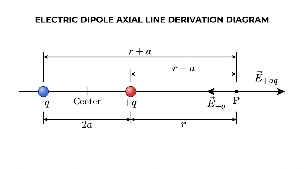
Derivation: Axial Line Let point $P$ be at a distance $r$ from the center of the dipole on its axis, towards the $+q$ side. Distance between charges is $2a$.
Field at P due to $+q$: $E_+ = \frac{1}{4\pi\epsilon_0} \frac{q}{(r-a)^2}$ (pointing away).
Field at P due to $-q$: $E_- = \frac{1}{4\pi\epsilon_0} \frac{q}{(r+a)^2}$ (pointing towards).
Net Field $E_{axial} = E_+ - E_-$ $= \frac{q}{4\pi\epsilon_0} \left[ \frac{1}{(r-a)^2} - \frac{1}{(r+a)^2} \right]$
$E_{axial} = \frac{q}{4\pi\epsilon_0} \left[ \frac{(r+a)^2 - (r-a)^2}{(r^2-a^2)^2} \right]$
$= \frac{q}{4\pi\epsilon_0} \left[ \frac{4ar}{(r^2-a^2)^2} \right]$
Since $p = q \times 2a$, we get $E_{axial} = \frac{1}{4\pi\epsilon_0} \frac{2pr}{(r^2-a^2)^2}$.

For a short dipole ($r \gg a$), $a^2$ is negligible: $$E_{axial} \approx \frac{1}{4\pi\epsilon_0} \frac{2p}{r^3}$$ The direction of $E_{axial}$ is the SAME as the dipole moment $\vec{p}$.

Electric Field due to a Dipole on the Equatorial Line (Broad-side on)

Electric Dipole Equatorial Field Derivation

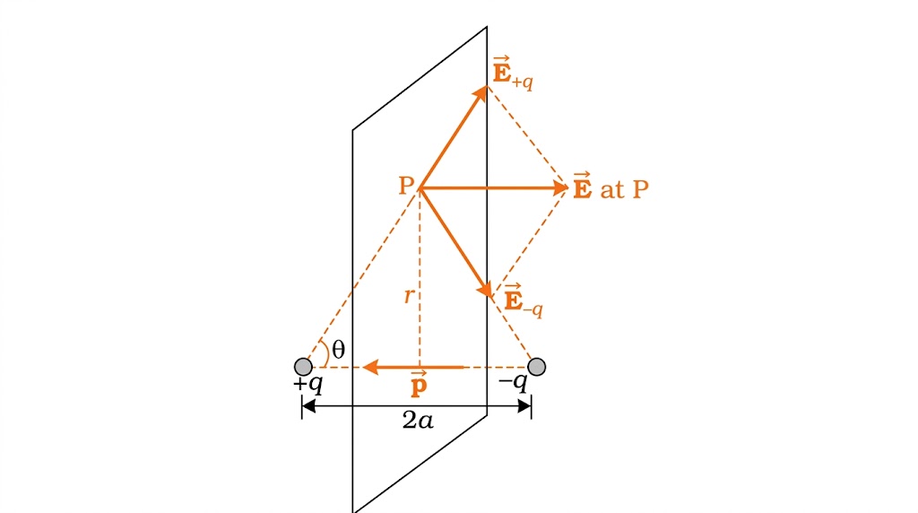
Derivation: Equatorial Line Let point $P$ be on the perpendicular bisector at a distance $r$ from the center.
Distance of P from both $+q$ and $-q$ is $\sqrt{r^2 + a^2}$.
$E_+ = E_- = \frac{1}{4\pi\epsilon_0} \frac{q}{(r^2+a^2)}$.
Resolving into components, the vertical ($\sin\theta$) components cancel out. The horizontal ($\cos\theta$) components add up.
$E_{eq} = 2 E_+ \cos\theta$. From the geometry triangle, $\cos\theta = \frac{a}{\sqrt{r^2+a^2}}$.
$E_{eq} = 2 \left( \frac{1}{4\pi\epsilon_0} \frac{q}{(r^2+a^2)} \right) \left( \frac{a}{\sqrt{r^2+a^2}} \right)$
$= \frac{1}{4\pi\epsilon_0} \frac{q \times 2a}{(r^2+a^2)^{3/2}}$

For a short dipole ($r \gg a$): $$E_{eq} \approx \frac{1}{4\pi\epsilon_0} \frac{p}{r^3}$$ The direction of $E_{eq}$ is OPPOSITE to the dipole moment $\vec{p}$.
Crucial Relation: $E_{axial} = 2 \times E_{eq}$

6. Dipole in a Uniform Electric Field

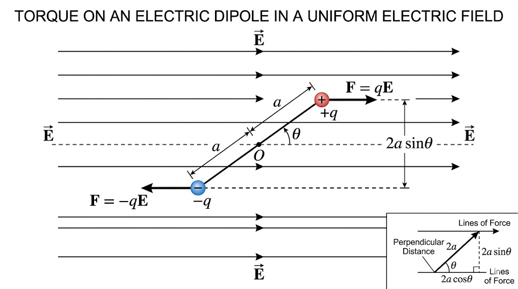
When a dipole is placed in a uniform electric field $\vec{E}$ at an angle $\theta$, the net force on the dipole is exactly zero ($+qE$ and $-qE$ cancel out). However, these two equal, opposite, and non-collinear forces form a Couple, which exerts a Torque ($\vec{\tau}$) trying to align the dipole with the field.

Torque and Potential Energy Torque = Force $\times$ Perpendicular distance between forces.
$\tau = (qE) \times (2a \sin\theta) = (q \times 2a) E \sin\theta$
$$\tau = pE \sin\theta \quad \implies \quad \vec{\tau} = \vec{p} \times \vec{E}$$
Potential Energy ($U$): The work done by an external agent in rotating the dipole against the electrostatic torque is stored as potential energy.
$dW = \tau d\theta = pE \sin\theta d\theta \implies U = \int_{90^\circ}^{\theta} pE \sin\theta d\theta$
$$U = -\vec{p} \cdot \vec{E} = -pE \cos\theta$$

Equilibrium Conditions:

Stable Equilibrium ($\theta = 0^\circ$): Dipole is aligned perfectly with the field. Torque is 0. Potential Energy is Minimum ($U = -pE$). If disturbed slightly, it naturally oscillates back to $0^\circ$.
Unstable Equilibrium ($\theta = 180^\circ$): Dipole is anti-aligned. Torque is 0. Potential Energy is Maximum ($U = +pE$). If disturbed even slightly, it violently flips completely over.

Practice Problem 3 Question: An electric dipole with dipole moment $4 \times 10^{-9} \text{ C}\cdot\text{m}$ is aligned at $30^\circ$ with the direction of a uniform electric field of magnitude $5 \times 10^4 \text{ N/C}$. Calculate the magnitude of the torque acting on the dipole and the work done to rotate it from $30^\circ$ to $90^\circ$.

Solution:
Given: $p = 4 \times 10^{-9}$, $E = 5 \times 10^4$, $\theta = 30^\circ$.
1. Torque: $\tau = pE \sin\theta$ $= (4 \times 10^{-9}) \times (5 \times 10^4) \times \sin 30^\circ$
$\tau = (20 \times 10^{-5}) \times 0.5 = \mathbf{10^{-4} \text{ N}\cdot\text{m}}$.

2. Work Done: $W = U_{final} - U_{initial}$
$= (-pE \cos\theta_2) - (-pE \cos\theta_1)$
$= pE(\cos\theta_1 - \cos\theta_2)$ where $\theta_1 = 30^\circ$ and $\theta_2 = 90^\circ$.
$W = (20 \times 10^{-5})(\cos 30^\circ - \cos 90^\circ)$ $= (20 \times 10^{-5})(\frac{\sqrt{3}}{2} - 0)$
$W = 10\sqrt{3} \times 10^{-5} = \mathbf{1.732 \times 10^{-4} \text{ Joules}}$.

7. Continuous Charge Distribution

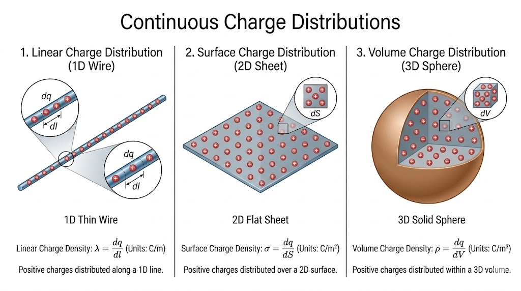
At macroscopic scales, we ignore the discrete quantized nature of charge and treat it as a continuous spread over lines, surfaces, or volumes. The electric field is calculated using integration: $\vec{E} = \frac{1}{4\pi\epsilon_0} \int \frac{dq}{r^2} \hat{r}$.

Linear Charge Density ($\lambda$): Charge per unit length. $dq = \lambda dl$. Unit: $\text{C/m}$.
Surface Charge Density ($\sigma$): Charge per unit area. $dq = \sigma dS$. Unit: $\text{C/m}^2$.
Volume Charge Density ($\rho$): Charge per unit volume. $dq = \rho dV$. Unit: $\text{C/m}^3$.

8. Electric Flux and Gauss's Law

A. Electric Flux ($\Phi_E$) and Area Vector

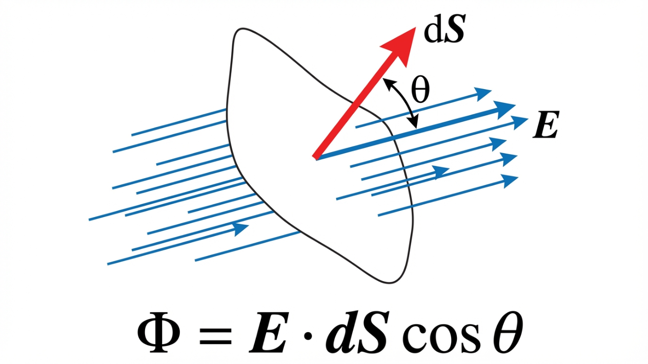
In electrostatics, we treat an area as a vector quantity. The Area Vector ($d\vec{S}$) always points perpendicular (outward normal) to the surface.

Electric flux linked with any surface is the total number of electric field lines crossing normally through that surface. It is the dot product of the Electric Field vector and the Area vector.

$$\Phi_E = \oint \vec{E} \cdot d\vec{S} = \oint E \, dS \cos\theta$$

Flux is a Scalar quantity. SI Unit: $N \cdot m^2/C$ or $V \cdot m$.

B. Gauss's Law (Statement and Proof)

Gauss's Theorem "The total electric flux through any closed surface (Gaussian surface) in free space is equal to $1/\epsilon_0$ times the net charge enclosed by the surface." $$\Phi_{total} = \oint \vec{E} \cdot d\vec{S} = \frac{q_{enclosed}}{\epsilon_0}$$

Formal Proof from Coulomb's Law:
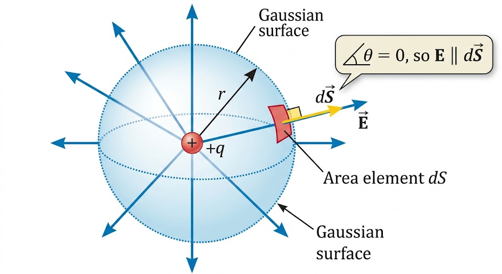
Imagine a point charge $+q$ at the center of a spherical Gaussian surface of radius $r$.
At any point on the sphere, the electric field is $\vec{E} = \frac{1}{4\pi\epsilon_0} \frac{q}{r^2} \hat{r}$.
The area vector $d\vec{S}$ also points radially outward, so the angle between $\vec{E}$ and $d\vec{S}$ is $0^\circ$ ($\cos 0^\circ = 1$).
Flux $\Phi_E = \oint \vec{E} \cdot d\vec{S} = \oint E \, dS \cos(0^\circ) = \oint E \, dS$
Since $r$ is constant over the sphere, $E$ is constant and can be pulled out of the integral:
$\Phi_E = E \oint dS$
The total surface area of a sphere $\oint dS = 4\pi r^2$.
$\Phi_E = \left(\frac{1}{4\pi\epsilon_0} \frac{q}{r^2}\right) \times (4\pi r^2)$
$\Phi_E = \frac{q}{\epsilon_0}$. (Hence Proved!).

Important Conceptual Points:

Gauss's law is true for any closed surface, no matter what its shape or size.
The charge $q_{enclosed}$ includes the sum of all charges located inside the surface. Charges outside the surface do NOT contribute to the total net flux.
However, the electric field $\vec{E}$ in the integral $\oint \vec{E} \cdot d\vec{S}$ is the net electric field due to ALL charges, both inside and outside the surface.

9. Applications of Gauss's Law (High Probability Board Long Answers)

1. Field due to an Infinitely Long Straight Uniformly Charged Wire

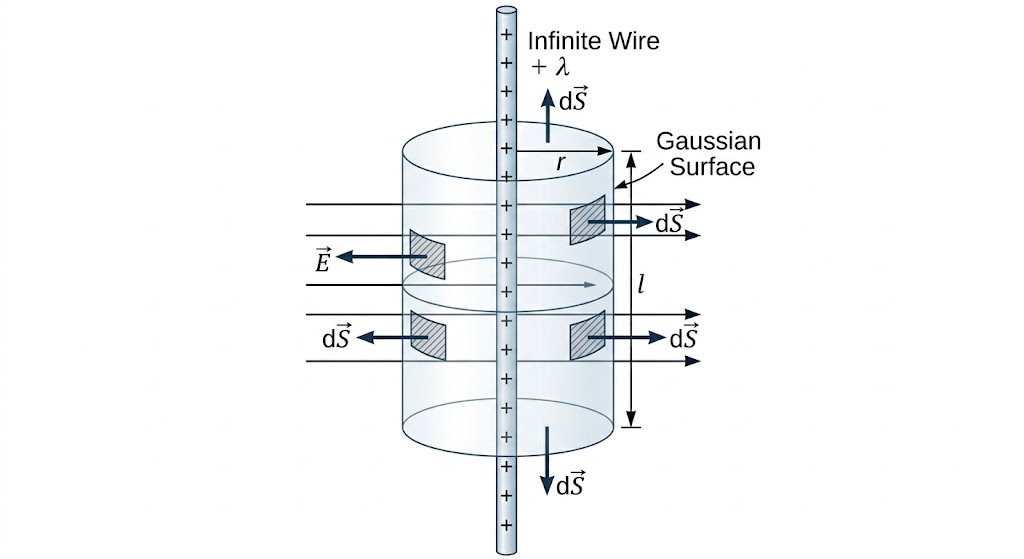
Consider an infinite wire with linear charge density $\lambda$. We choose a cylindrical Gaussian surface of radius $r$ and length $l$ coaxial with the wire.

The flux through the two flat circular caps is zero because $\vec{E}$ and $d\vec{S}$ are perpendicular ($\cos 90^\circ = 0$).
The flux through the curved surface: $\oint \vec{E} \cdot d\vec{S} = E \oint dS = E(2\pi rl)$ (since $\vec{E}$ is parallel to $d\vec{S}$, $\cos 0^\circ = 1$).
By Gauss's Law: $E(2\pi rl) = \frac{q_{encl}}{\epsilon_0}$.
Since $q_{encl} = \lambda l$, we get $E(2\pi rl) = \frac{\lambda l}{\epsilon_0}$.

Formula $$E = \frac{\lambda}{2\pi\epsilon_0 r}$$ The electric field is inversely proportional to the distance $r$ ($E \propto 1/r$).

2. Field due to a Uniformly Charged Infinite Plane Sheet

Consider an infinite sheet with surface charge density $\sigma$. We choose a cylindrical pillbox Gaussian surface passing horizontally through the sheet, with cross-sectional area $A$.

The flux through the curved surface is zero ($\vec{E} \perp d\vec{S}$). Flux passes only through the two flat end caps where $\vec{E} \parallel d\vec{S}$.
Total Flux = $EA (\text{left cap}) + EA (\text{right cap}) = 2EA$.
The charge enclosed inside the pillbox is $q_{encl} = \sigma A$.
By Gauss's Law: $2EA = \frac{q_{encl}}{\epsilon_0} = \frac{\sigma A}{\epsilon_0}$.

Formula $$E = \frac{\sigma}{2\epsilon_0}$$ Crucial Fact: The electric field is UNIFORM. It does NOT depend on the distance $r$ from the sheet!

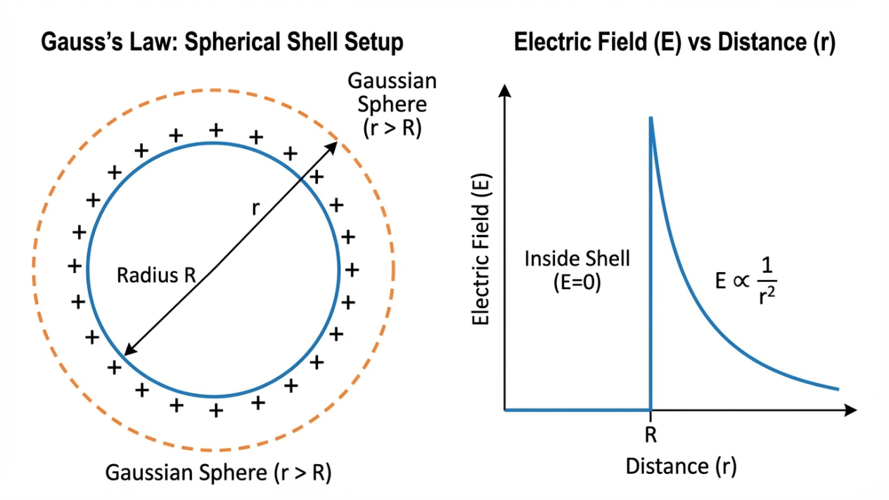
3. Field due to a Uniformly Charged Thin Spherical Shell

Consider a shell of radius $R$ with total charge $q$ spread uniformly over its surface ($\sigma = q / 4\pi R^2$).

Case A: Outside the shell ($r > R$)
Gaussian surface is a sphere of radius $r$. $\oint E \, dS = E(4\pi r^2) = \frac{q}{\epsilon_0}$.
$E = \frac{1}{4\pi\epsilon_0} \frac{q}{r^2}$. (It behaves exactly as if all its charge is concentrated at the center).

Case B: On the surface ($r = R$)
$E = \frac{1}{4\pi\epsilon_0} \frac{q}{R^2} = \frac{\sigma}{\epsilon_0}$.

Case C: Inside the shell ($r < R$)
Gaussian surface is a sphere of radius $r$ inside the shell. Enclosed charge $q_{encl} = 0$ because all charge resides on the outer surface.
Therefore, $\oint E \, dS = 0 \implies$ $E = 0$. (This is the principle of Electrostatic Shielding!).

Practice Problem 4: JEE Main Parallel Sheets Question: Two infinite parallel plane sheets have uniform surface charge densities $+\sigma$ and $-\sigma$ respectively. Determine the electric field (i) in the region between the sheets, and (ii) in the regions outside the sheets.

Solution:
Let Sheet 1 have $+\sigma$ and Sheet 2 have $-\sigma$. Magnitude of field due to one sheet is $E = \sigma / 2\epsilon_0$.

(i) In the region between the sheets:
The field due to $+\sigma$ points away from Sheet 1 (towards Sheet 2).
The field due to $-\sigma$ points towards Sheet 2 (which is the same direction).
Since they point in the same direction, they add up: $E_{net} = \frac{\sigma}{2\epsilon_0} + \frac{\sigma}{2\epsilon_0} = \mathbf{\frac{\sigma}{\epsilon_0}}$.
(This is the foundational principle for Parallel Plate Capacitors in Chapter 2!)

(ii) In the regions outside the sheets:
Outside either sheet, the field from $+\sigma$ points away, and the field from $-\sigma$ points towards the sheet. They point in opposite directions with equal magnitudes.
Therefore, $E_{net} = \frac{\sigma}{2\epsilon_0} - \frac{\sigma}{2\epsilon_0} = \mathbf{0}$.